Amortized Analysis
1. What is it?
Amortized: paid-off over time.
The time required to perform a sequence of data structures operations is averaged over all operations performed.
This guarantees the average performance of each operation in the worst case (meaning, we take the worst case performance of each operation and average the total).
This is ==not the same== as average case analysis which relies on some probability distribution of the input while amortized always considers the worst case.
2. Why amortized analysis?
- Can be used to show that the average cost of an operation is small, even though a single operation can be costly.
- Extra flexibility of amortized bounds can lead to more practical data structures. e.g. balanced binary search tree (usually, we need to rebalance the tree after insertion/deletion operations) vs. splay tree.
3. Aggregate analysis
Steps
- Show that for all $n$, a sequence of $n$ operations uses $T(n)$ worst-case time.
- The amortized cost per operation is $\frac{T(n)}{n}$.
Each operation has the same amortized cost.
Example: Stack with multi-pop
Problem: $MULTIPOP(S, k)$ given the stack $S$, remove its $k$ top objects.
Pseudocode:
While $k \neq 0$ and not $STACK-EMPTY(S)$ do $POP(S)$ $k \leftarrow k-1$
Worst-case analysis: PUSH, POP: $O(1)$ MULTIPOP: $O(\min(k,s))$ given that the stack initially contains $s$ elements.
Aggregate Analysis
Analysis of a sequence of $n$ PUSH, POP, and MULTIPOP operations on an initially empty stack.
MULTIPOP: $O(n) \rightarrow$ the worst case of any operation is $O(n) \rightarrow$ the total cost of $n$ operations is $O(n^2)$. ==This is not tight!==
Proper analysis: Observation: each object can be popped at most once for each time it is pushed.
The number of times POP can be called on an initially-empty stack, including calls within MULTIPOP, is at most the number of PUSH operations $\rightarrow$ which is $O(n)$.
The total cost of $n$ PUSH, POP, MULTIPOP operations on an initially empty stack is $O(n)$.
Amortized cost per operation: $\frac{O(n)}{n} = O(1)$.
Example: Incrementing a Binary Counter
Problem: A $k$-bit binary counter that counts upward from $0$. Stored in an array $A[0 \dots k-1]$.
Example: Let $k=5$, array $=01011$. Incrementing this turns it into $01100$.
Procedure:
==Shows us that the running time is proportional to the number of bit flips.==
INCREMENT($A[0 \dots k-1]$) i $\rightarrow$ 0 While $i < k$ and $A[i] = 1$ do $A[i] \rightarrow 0$ $i \rightarrow i+1$ If $i < k$ then $A[i] \rightarrow 1$
Worst-case analysis: INCREMENT: $O(k)$ $n$ INCREMENTS: $O(kn)$
Example:
| Value | A[4] | A[3] | A[2] | A[1] | A[0] |
|---|---|---|---|---|---|
| 0 | 0 | 0 | 0 | 0 | 0 |
| 1 | 0 | 0 | 0 | 0 | 1 |
| 2 | 0 | 0 | 0 | 1 | 0 |
| 3 | 0 | 0 | 1 | 1 | 1 |
| 4 | 0 | 0 | 1 | 0 | 1 |
| ==Observation:== $A[0]$ flips every time INCREMENT is called, $A[1]$ flips every other time, A[2], flips every third time, etc. | |||||
| $\rightarrow$ For $i=0, 1, \dots \lfloor \log n \rfloor$, bit $A[i]$ flips $\lfloor \frac{n}{2^i}\rfloor$ times in a sequence of $n$ INCREMENT operations on an initially $0$ counter. | |||||
| $\rightarrow$ For $i > \lfloor \log n \rfloor$, bit $A[i]$ never flips. |
We can use the above observations to conclude that the total number of bit flips in the sequence of $n$ INCREMENT operations is $$\sum_{i=0}^{\lfloor \log n \rfloor} \left\lfloor \frac{n}{2^i} \right\rfloor < \sum_{i=0}^\infty \frac{n}{2^i} = n\sum_{i=0}^\infty \frac{1}{2^i} = 2n \quad \text{(Geometric series)}$$ Worst-case analysis: the worst-case time of a sequence of $n$ INCREMENT operations in thus $O(n)$.
Amortized cost per operation: $\frac{O(n)}{n} = O(1)$.
3. The accounting method
Idea: We pre-charge a cost for each operation, and we need to make sure that there is enough "credit" for each operation.
Steps:
-
We charge each operation what we think its amortized time =="cost"== is.
-
- If the amortized cost exceeds the actual cost, the surplus remains as a =="credit"== associated with the data structure.
- If the amortized cost is less than the actual cost, the accumulated credit is used to pay for the cost overflow.
$\rightarrow$ To show that the amortized cost is correct, we should ensure that, at all times the total credit associated with the data structure is nonnegative $\iff$ the total amortized cost $\geq$ the total actual cost.
==Why is this enough:== The credit is the difference between the total amortized cost so far, and the total actual cost so far.
Example: Stack with MULTIPOP
Recall that Actual cost: PUSH is $O(1)$ ($1$ dollar), POP is $O(1)$ ($1$ dollar) and MULTIPOP is $O(\min(k, s))$ ($\min(k, s)$ dollars) where $s$ is the number of items in the stack.
Suppose we assign the following amortized costs: PUSH $\rightarrow$ $2$ dollars POP $\rightarrow$ $0$ dollars MULTIPOP $\rightarrow$ $0$ dollars (resulting in $O(1)$ amortized time).
We start with an empty stack, whose credit is $0$, which is fine because it is nonnegative.
When we PUSH an object into the stack, we charge the operation $2$ dollars. Since this results in an excess cost of $1$, we charge $1$ dollar and use the other as credit. ==We associate this credit with the object we just pushed onto the stack.==
When we POP an object from the stack, we ==thus charge the operation nothing== as we pay its cost using its $1$ dollar credit. Since each object pushed onto the stack is associate with a credit, POP will never make the credit negative.
And the same analysis applies for MULTIPOP$(k,s)$. There are $\min(k,s)$ dollars of credit associated with $\min(k,s)$ objects being popped. Therefore, the total credit of the stack is nonnegative at all times.
Example: Incrementing a binary counter
The running time of INCREMENT is proportional to the number of bits flipped, and the actual cost of bit flipping is $1$ dollar.
Suppose we charge a bit flip of $0 \rightarrow 1$ an amortized cost of $2$ dollars and a bit flip of $1 \rightarrow 0$ a cost of $0$ dollars which we associate with the flipped bit.
Therefore, when we flip $1$ to $0$, we charge $1$ dollar and give that bit $1$ dollar of credit.
Since all the bits are initially $0$s, the total credit of the binary counter is initially $0$ and therefore nonnegative. Moreover, we can conclude that it is nonnegative at all times.
INCREMENT changes at most one $0$ bit to $1$, so ==its amortized cost is at most== $2$, ==which results in $O(1)$!==
4. The Potential Method
Idea: Instead of credits, we present the prepaid work as ==potential== which can be ==released== to pay for future operations.
What's the difference between this and the credit system? Potential is a ==function== of the entire data structure.
Steps
- Let $D_{i}$ be our data structure after the $i$th operation and
- Let $\phi(D_{i})$ be the potential of $D_{i}$ and
- Let $C_{i}$ be the cost of the $i$th operation
- The amortized cost of the $i$th operation $a_{i} = C_{i} + \phi(D_{i}) - \phi(D_{i-1})$
$\rightarrow$ $\phi(D_{i}) - \phi(D_{i-1})$ is the change in potential
A correct potential function ensures that the total amortized cost is an upper bound on the total actual cost.
The total amortized cost of $n$ operations is $$\sum_{i=1}^n a_{i} = \sum_{i=1}^n(C_{i} + \phi(D_{i}) - \phi(D_{i-1})) = (\sum_{i=1}^n C_{i}) + \phi(D_{n}) - \phi(D_{0})$$ ==Our task now is to define a potential function such that==
- $\phi(D_{0}) = 0$
- $\phi(D_{i}) \geq 0$ for all $i$
If we achieve, we guarantee the upper bound $$\sum_{i=1}^n C_{i} = \sum_{i=1}^n a_{i} - \phi(D_{n}) \leq \sum_{i=1}^n a_{i}$$ Example: Stack with MULTIPOP
We define the potential function $\phi$ on an initially empty stack to be the ==number of objects== in the stack. Therefore, $\phi(D_{0}) = 0$ where $D_{0}$ is the empty stack. This definition also ensures that the potential is always nonnegative as we can never have a negative number of objects in the stack. Moreover, the total amortized cost of $n$ operations with respect to $\phi$ represents an upper bound on the actual cost.
If the stack contains $s$ objects before the $i$th operation, then PUSH leads to a positive change in potential of $1$ $$\phi(D_{i}) - \phi(D_{i-1}) = s + 1 - s = 1$$ And $$a_{i} = C_{i} +1$$ Similar logic applies if we do MULTIPOP with $k' = \min(k, s)$ elements, the change in potential would be $k'$ and the amortized cost of the $i$th operation is $C_{i} - k' = k'- k' = 0$.
$C_{i} = k'$ because the actual cost would be at most $k'$ elements popped by multipop.
And with pop, in that case the amortized cost would be $1 - 1 = 0$.
Example: Binary counter
We let $\phi(D_{i})$ be the number of set bits (the number of $1$s). We define this quantity as $b_{i}$.
This potential function is correct because, initially, no bits are set and so $\phi(D_{0}) = 0$. Moreover, it can never be negative as you cannot have a negative number of set bits.
The amortized cost of an INCREMENT operation will depend on the number of $1$s flipped to $0$s. Define this quantity for the $i$th increment as $t_{i}$.
The actual cost of the operation is, therefore, at most $t_{i}+1$.
If $b_{i}$ is $0$, then the $i$th operation sets all $k$ bits from $1$ to $0$. So, $b_{i-1} = t_{i} = k$.
If $b_{i} > 0$, then $b_{i}= b_{i-1} - t_{i} + 1$.
So, in either case, $b_{i} \leq b_{i-1} - t_{i} +1$, and the potential difference is $$ \begin{aligned} &= b_{i} - b_{i-1} \ &\leq (b_{i} - t_{i} +1)- b_{i-1} \ &= 1 - t_{i} \end{aligned} $$ And the amortized cost is therefore $$ \begin{aligned} a_{i} &= C_{i} + \phi(D_{i}) - \phi(D_{i-1}) \ &\leq (t_{i}+1)+ (1-t_{i}) \ &= 2 \ &=O(1) \ \end{aligned} $$
Entropy
1. Entropy
1. Definition
Given a set of objects $S = { k_{1}, \dots, k_{n} }$, a probability distribution for each object $D = { p_{1}, \dots , p_{n} }$, the entropy $H(D)$ of $D$ is $$-\sum_{i=1}^np_{i} \cdot \log(p_{i}) = \sum_{i=1}^n p_{i} \cdot \log\left( \frac{1}{p_{i}} \right)$$
2. Shannon's Theorem
Given a sender and a receiver, in which the sender want to send a sequence $S_{1}, \dots , S_{m}$ where each $S_{j}$ is chosen randomly and independently according to $D$, meaning that $S_{j} = k_{i}$ with probability $p_{i}$, Shannon's theorem states that for any protocol that the sender and the receiver might use, the expected number of bits required to transmit $S_{1}, \dots S_{m}$ using that protocol, which is at least $$m \cdot H(D)$$
3. Examples
If we have a uniform distribution $p_{i} = \frac{1}{n}$, then $$H(D) = \sum_{i=1}^n \left( \frac{1}{n} \right) \log (n) = \log (n) \quad \text{(worst case)}$$If we have a geometric distribution $p_{i} = \frac{1}{2^i}$ for all $1 \leq i < n$, then $$H(D) = \sum_{i=1}^{n-1} \frac{i}{2^i} + \frac{n-1}{2^{n-1}}$$ This is an arithmetico-geomtric series.
2. Entropy and data structure lower bounds
1. Theorem 1
For any comparison-based data structure storing $k_{1}, \dots , k_{n}$, each associated with probabilities $p_{1}, .., p_{n}$, the expected number of comparisons while searching for an item is $\Omega(H(D))$.
Proof
Assume that the sender and receiver both store the elements $k_{1}, \dots , k_{n}$ in some comparison-based data structure that is agreed on beforehand.
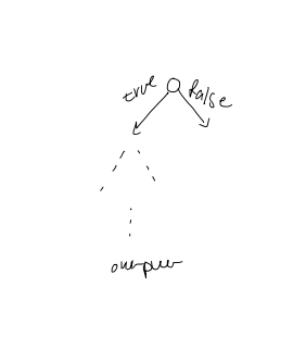
When the sender wants to transmit $S_{1}$, they perform the search for $S_{1}$ in the data structure. This results in a sequence of comparisons and the results of the comparisons form a sequence of $1$s (true) and $0$s (false) which the sender sends to the receiver.
On the receiving end, the receiver runs a search algorithm without knowing the value of $S_{1}$. This can be done since the receiver is doing exactly the same comparisons and knows the results of the comparisons. This way, the sender can transmit a sequence to the receiver.
Now, consider the number of bits needed to transmit this sequence and the number of comparisons needed to handle the request sequence, these numbers are the same.
2. Static optimal BST
Assume that all the elements in the request sequence are in the tree, that $p_{i}$ is the probability of access of the element $A_{i}$, and that the entropy $H = \sum_{i=1}^n p_{i} \cdot \log\left( \frac{1}{p_{i}} \right)$.
The expected cost (number of comparisons), $C$, of the static optimal BST is $\geq H$.
3. Not all requested elements are in the tree
Let $p_{i}$ be the probability of access of element $A_{i}$ and $q_{i}$ be the probability of requesting an element between $A_{i}$ and $A_{i+1}$. The entropy is defined as $$H = \sum_{i=1}^n p_{i} \cdot \log\left( \frac{1}{p_{i}} \right) + \sum_{i=0}^n q_{i} \cdot \log\left( \frac{1}{q_{i}} \right)$$ Note that $C \geq H$ still applies.
3. Nearly-Optimal Search Trees
1. $p_{i}, H$
Our goal is to achieve $O(H+1)$ query time. #final what is the point of the $+1$? Edge case of 1/log(n), etc.
2. Idea: Probability Splitting
First, we find a key $k_{i}$ such that $$\sum_{j=1}^{i-1}p_{j} \leq \frac{1}{2} \sum_{j=1}^n p_{j}$$And $$\sum_{j=i+1}^np_{j} \leq \frac{1}{2} \sum_{j=1}^n p_{j}$$
Let the key $k_{i}$ become the root of a binary search tree, then recurse.
So, the left subtree is constructed recursively from $(k_{1}, \dots k_{i-1})$ with probabilities $(p_{1}, \dots , p_{i-1})$ and the right subtree is constructed recursively from $(k_{i+1}, \dots k_{n})$ with probabilities $(p_{i+1}, \dots , p_{n})$.
Let $T$ be the resulting tree.
Observation: In $T$, if node $k_{i}$ has depth $\text{depth}T(k{i})$, then $$\sum_{k_{j}\in T(k_{i})}p_{j} \leq \frac{1}{2^{\text{depth}T(k{i})}}$$ Where $T(k_{i})$ is the set of nodes in the subtree rooted at $k_{i}$.
Theorem: $T$ can answer queries in $O(H + 1)$ expected time Proof: As $$p_{i} \leq \sum_{k_{j} \in T(k_{i})} p_{j} \leq \frac{1}{2^{\text{depth}T(k{i})}},$$ It must be true that $$\text{depth}T(k{i}) \leq \log\left( \frac{1}{p_{i}} \right).$$ Thus, the expected depth of a chosen key is $$\sum_{i=1}^n p_{i} \cdot \text{depth}T(k{i}) \leq \sum_{i=1}^n p_{i} \cdot \log\left( \frac{1}{p_i} \right) = H,$$ yielding a running time of $O(H+1)$.
Construction
- Finding $k_{i}$
This takes linear, $\Theta(n)$, time.
- $n$ keys
$\Theta(n^2)$?
Better algorithm
- Finding $k_{i}$
Use binary search instead, $\Theta(n \log n)$
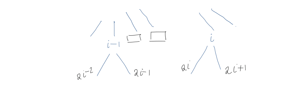
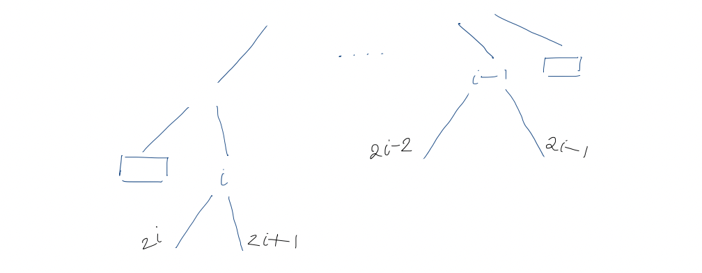
Best Algorithm*
- Finding $k_{i}$
Use doubling (exponential) search.
- Check $k_{1}, k_{2}, k_{4}, k_{8}, \dots$ until we find the first $k_{2}^j$ with $2^j \geq i$
- Binary search in $k_{2}^{j-1}, \dots, k_{2}^j$
This gives us a running time of $\Theta(\log n)$. In fact, it is $\Theta(\log i)$ because $2^j \leq 2i$.
Idea: search simultaneously starting at $k_{1}$ and working forward, and starting at $k_{n}$ and working backward.
Then, $k_{i}$ can be found in $O{(\log(\min(i, n-i +1)))}$.
And the total running time becomes $$T(n) = O(\log(\min (i, n-i +1))) + T(i-1) + T(n-i)$$Which we can prove, by induction that the running time is $O(n)$.
4. MTF Compression
1. Elias gamma coding
Used to code positive, and sometimes, negative integers whose maximum value is not known. There are $i \geq 0$ steps of encoding.
-
Write down the binary expression of $i$, which uses $\log \lfloor i \rfloor + 1$ bits
-
Prepend it by $\lfloor \log i \rfloor$ $0$'s
Example: $9 \rightarrow 0001001$
2. A coding scheme that uses fewer bits:
-
Gamma code: the leading $0$s encode $\lfloor \log i \rfloor \leq \log i$
-
This number can be encoded using $2\lfloor \log \log i \rfloor + 1$ bits using Elias gamma coding
Example: $9 \rightarrow 0111001$
So, the number of bits used is $\log i + O(\log \log i)$.
3. MTF Compression
Encode $m$ integers from $1$ to $m$.
-
The sender and receiver each maintain identical lists of $1, 2, \dots, n$
-
To send the symbol $j$ we do not encode $j$ directly. Instead, the sender looks for $j$ in their list and finds it at position $i$.
-
Sender encodes $i$ in $\log i + O(\log \log i)$ bits and sends them to the receiver
-
The receiver decodes $i$, and looks at the $i$th element in the list to find $j$
-
Both move $j$ to the front and continue
Example: Given the range $1, 2$ 2211112 21211122
Jensen's inequality: Let $f: R \rightarrow R$ be a strictly increasing concave function. Then, $\sum_{i=1}^n f(t_{i})$ subject to $\sum_{i=1}^nt_{i} \leq m$ is maximized when $t_{1} = t_{2} = \dots = t_{n} = \frac{m}{n}$.
Claim: We can use this to prove that $\text{MTF}$ compresses $S_{1}, \dots S_{m}$ into $$n \log n + m\cdot H + O(n \log \log n + m \log H)$$ bits.
Proof: If the number of distinct symbols between two consecutive occurrences of $j$ is $t-1$, then the cost of encoding the second $j$ is $\log(t) + O(\log \log t)$. Therefore, the total cost of encoding all the occurrences of $j$ is
- #final Where does the $n + O(n \log n)$ term come from? And how do the $t$s stay constant if we are employing MTF? $$\begin{gathered} C_{j} \leq \log n + O(\log \log n) + \sum_{i=1}^{m_{j}}(\log t_{i} + O(\log \log t_{i})) \ & \left( \sum_{j=1}t_{j} \leq m \right)\ \leq \log n + O(\log \log n) + m_{j}\left( \log\left( \frac{m}{m_{j}} \right) + O\left( \log \log \frac{m}{m_{j}} \right) \right) \end{gathered}$$ Where $t_{i} - 1$ is the number of symbols between the $i-1$ and $i$ occurrence of $j$.
Summing over all $j$, the total number of bits used is
$$\begin{aligned} &\sum_{j=1}^n C_{j}\ &\leq n \log n + O(n \log \log n) + m \cdot H + \sum_{j=1}^m O\left( m_{j} \log \log \frac{m}{m_{j}} \right) \ & \leq n \log n + m \cdot H + O(n \log \log n + m \log H) \end{aligned}$$
Resizable Arrays
Definition: A resizable array $A$ represents $n$ fixed-size elements, each assigned a unique index from $0$ to $n-1$ to support $\text{Locate}(i)$: determines the location of $A[i]$ $\text{Insert}(x):$ store $x$ in $A[n]$, and increment $n$ $\text{Delete}$: discard $A[n-1]$, decrementing $n$
Vector?
- No deletion
Strategy: upon inserting an element into a full array, allocate a new array with twice the size, and copy all the elements, including the new one, over. Define: $n$: the number of elements in $A$ $s$: the capacity of $A$ Load factor $\alpha = \frac{n}{s}$ when $A$ is nonempty, and $=1$ otherwise. $\alpha$ is always $\geq \frac{1}{2}$
Pseudocode: $\text{Insert}(x)$: If $s=0$ allocate $A$ with $1$ slot $s \leftarrow 1$ If $n=s$ allocate $A'$ with $2s$ slots copy all elements of $A$ into $A'$ deallocate $A$ $A' \leftarrow A$ $s \leftarrow 2s$ $A[n] \leftarrow x$ $n \leftarrow n+1$
Cost analysis: Insert If $A$ is not full for the $it$th insert, we simply copy one element, and the cost is $1$. Otherwise, the cost is $i$ because we copy $i$ elements.
[[Amortized Analysis]]: Let $A_{i}$ denote the array $A$ after the $i$th insert. What should we define our potential as? Idea 1: $\phi(A_{i}) = n$ Problem: $\phi(A_{i}) - \phi(A_{i-1}) = 1$ Idea 2: $\phi(A_{i}) = n-s$ Problem: $\phi(A_{i}) \leq 0$ Idea 3: $\phi(A_{i}) = 2n - s$ $\phi(A_{0}) = 0$ And $\phi(A_{i}) \geq 0$ for all $i$ ==Good!==
To analyze the amortized cost, $a_{i}$, of the $i$th insert, let $n_{i}$ denote the number of elements stored in $A_{i}$ and $S_{i}$ denote the total size of $A_{i}$.
Now, we need to consider two cases: 1. The $i$th insert does not require the array to be reallocated Then $S_{i} = S_{i-1}$ Thus, $$\begin{aligned}a_{i} &= C_{i} + \phi(A_{i}) - \phi(A_{i-1})\ &= 1 + (2n_{i} - S_{i}) - (2n_{i-1} - S_{i-1}) \ &= 1 + (2(n_{i-1} + 1) - s_{i-1}) - (2n_{i-1} - S_{i-1}) \ &= 3\end{aligned} $$ 2. The $i$th insert requires a new array to be allocated. Then $S_{i} = 2S_{i-1}$ and $S_{i-1} = n_{i-1}$ And thus $$\begin{aligned}a_{i} &= C_{i} + \phi(A_{i}) - \phi(A_{i-1}) \ &= n_{i} + (2n_{i} - s_{i}) - (2n_{i-1} - S_{i-1})\ &= n_{i-1} + 1 + (2(n_{i-1} + 1) - 2n_{i-1}) - (2n_{i-1} - n_{i-1}) \ &= 3 \end{aligned}$$
Therefore, the insert operation is $O(1)$ amortized time.
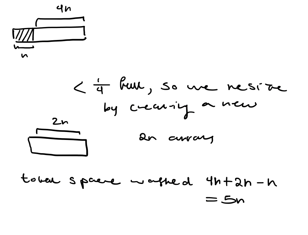
What about Delete? Idea 1: When $\alpha$ is too small, allocate a new, smaller array and copy the elements from the old array to the new array. Problem: Would not achieve $O(1)$ amortized time. Idea 2: Double the array size when inserting into a full array, halve the array size when deletion would cause the array to be less than half-full. Counterexample: For simplicity, assume $n$ is a power of $2$. The first $\frac{n}{2}$ operations are insertions, which cause $A$ to be full. The next $\frac{n}{2}$ are insert, then two deletes, then two inserts, two deletes, etc. Leading us to spend $\Theta(n)$ time every two operations, and an overall running time of $\Theta(n^2)$ Idea 3: We need to introduce more slack, what if we only half the size of the array when a deletion causes the array to be less than a quarter-full?
Analysis: Define $\alpha_{i}$ to be the load factor after the $i$th operation $$\phi(A_{i}) = \begin{cases} 2n_{i} - S_{i} \quad \text{if} \quad \alpha_{i} \geq \frac{1}{2} \ \ \frac{S_{i}}{2} - n_{i} \quad \text{if} \quad \alpha_{i} < \frac{1}{2} \ \end{cases}$$ We now consider two cases: 1. The $i$th operation is insert (exercise: what four cases did we eliminate here?) 1. $\alpha_{i-1} \geq \frac{1}{2}$ and a new array is allocated 2. $\alpha_{i-1} \geq \frac{1}{2}$ and no new array is allocated 3. $\alpha_{i-1} < \frac{1}{2}$ and $\alpha_{i} < \frac{1}{2}$ 4. $\alpha_{i-1} < \frac{1}{2}$ and $\alpha_{i} \geq \frac{1}{2}$ 2. The $i$th operation is delete 1. $\alpha_{i-1} < \frac{1}{2}$ and a new array is allocated 2. $\alpha_{i-1} < \frac{1}{2}$ and no new array is allocated 3. $\alpha_{i-1} \geq \frac{1}{2}$ and $\alpha_{i} \geq \frac{1}{2}$ 4. $\alpha_{i-1} \geq \frac{1}{2}$ and $\alpha_{i} < \frac{1}{2}$
Let's do case 2.1 $n_{i} = n_{i-1} - 1$ $S_{i-1} = 4n_{i-1}$ $S_{i} = \frac{S_{i-1}}{2} = 2n_{i-1}$ $\alpha_{i} = \frac{n_{i}}{S_{i}} = \frac{n_{i-1} - 1}{2n_{i-1}} < \frac{1}{2}$ $a_{i} = C_{i} + \phi(A_{i}) - \phi(A_{i-1})$ $= n_i + \frac{S_{i}}{2} - n_{i} - \left( \frac{S_{i-1}}{2} - n_{i-1} \right)$ $= (n_{i} -1) + n_{i-1} - (n_{i-1} -1) - 2n_{i-1} + n_{i-1}$ $= 0$
Why do we have a factor of $\frac{1}{2}$ in our piecewise definition of $\phi(A_{i})$? Try $C(S_{i} - 2n_{i})$ where $C$ is a constant and show why $\frac{1}{2}$ is the best.
Overhead: The overhead of a data structure currently storing $n$ elements is the amount of memory usage beyond the minimum required to store $n$ elements.
Example: Vector
Lower bound
Claim: At some point in time, $\Omega({\sqrt{ n }})$ overhead is necessary for any data structure that supports ==inserting== elements and ==locating== any of those elements in some order, where $n$ is the ==number of elements currently stored in the data structure.==
Proof: Consider the following sequence of operations for any $n$:
$Insert(a_{1}), Insert(a_{2}), Insert(a_{3}), \dots Insert(a_{n})$
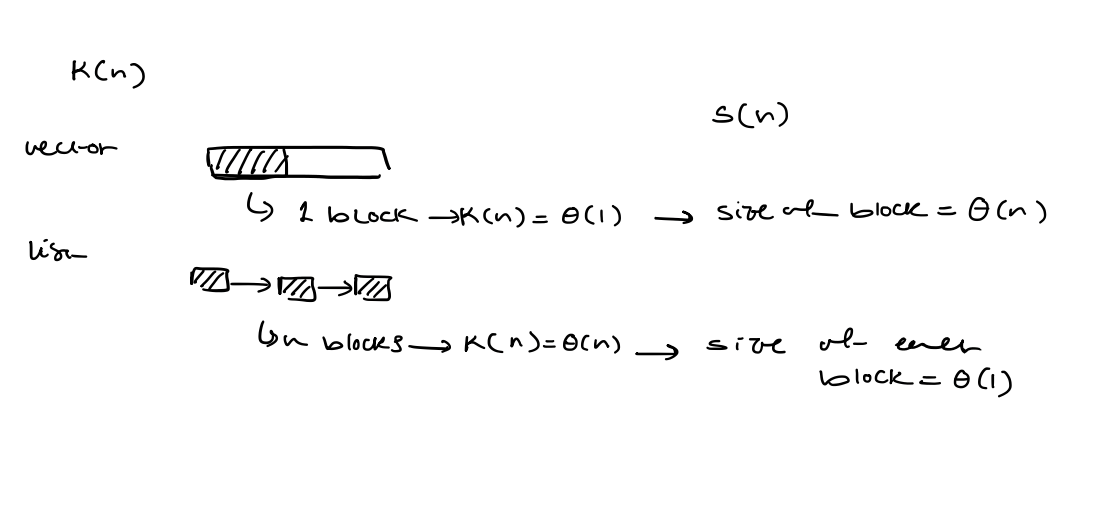
After inserting $a_{n}$, let $k(n)$ be the number of memory blocks occupied by the data structure and $S(n)$ be the size of the largest of those blocks. Hence, $S(n)\cdot k(n) \geq n$.
 At this time, the overhead is at least $k(n)$ to store bookkeeping information (e.g. address) for each block.
Furthermore, after the allocation of the block of size $S(n)$, the overhead is at least $S(n)$
The worst-case overhead is at least $\max(S(n), k(n))$.
Since $S(n) \cdot k(n) \geq n$, at some point, the overhead is at least $\sqrt{ n }$ (==because like we just stated, the overhead is the larger of the two and their product is larger than $n$)==.
At this time, the overhead is at least $k(n)$ to store bookkeeping information (e.g. address) for each block.
Furthermore, after the allocation of the block of size $S(n)$, the overhead is at least $S(n)$
The worst-case overhead is at least $\max(S(n), k(n))$.
Since $S(n) \cdot k(n) \geq n$, at some point, the overhead is at least $\sqrt{ n }$ (==because like we just stated, the overhead is the larger of the two and their product is larger than $n$)==.
An optimal solution Model: RAM $Allocate(S)$: Returns a new block of size $S$. $\rightarrow O(1)$ ($O(s)$ if initialization required) $Deallocate(B)$: Free the space used by the given block. $B$ $\rightarrow O(1)$ ($O(s)$ if initialization required) $Reallocate(B, S)$: If possible, resize block $B$ to size $S$. Otherwise, allocate a block of size $S$, copy the content of $B$ into a new block, and deallocate $B$. $\rightarrow O(s)$
Two approaches that do not work
- Try to store elements in $\theta(\sqrt{ n })$ blocks, where the size of the largest block is $\theta(\sqrt{ n })$
Issues: $locate(i)$: the element is in the $\left\lceil \frac{\sqrt{ 1 + 8i } - 1}{2} \right\rceil$th block and the ==RAM model is not naturally equipped with $\sqrt{ x}$.==
$locate(i)$ Block: number of bits in ($i+1$)$_{2} - 1$ Issue: the size of the largest block is $\theta(n)$
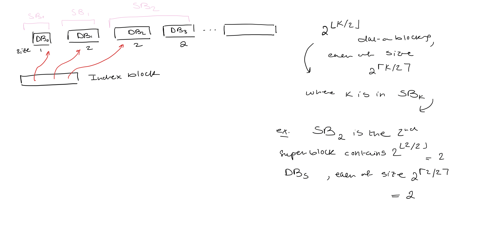
Solution: combine two ideas Index block: Data blocks: - Index block: pointers to data blocks - Data blocks $(DB_{0}, DB_{1}, \dots, DB_{d-1})$: elements - Super blocks $(SB_{0}, SB_{1}, SB_{s-1})$ - Data blocks are grouped into super blocks - Data blocks in the same superblock are of the same size - When $SB_{k}$ is fully allocate, it consists of $2^{\lfloor k/2\rfloor}$ data blocks, each of size $2^\left\lceil \frac{k}{2} \right\rceil$ - Size of $SB_{k}$ is $2^k$ - Only $SB_{s-1}$ might not be fully allocated
 Locate($i$)
$\rightarrow$ Let $r$ denote the binary expression of $i+1$ without leading $0$s. $\rightarrow$ Element $i$ is element $e$ of data block $b$ of superblock $k$. $\rightarrow$ $k = |r|-1$ $\rightarrow$ $b$ is $\left\lfloor \frac{k}{2} \right\rfloor$ bits of $r$ immediately after the leading $1$ bit $\rightarrow$ $e$ is the last $\left\lceil \frac{k}{2} \right\rceil$ bits of $r$ $\rightarrow$ The number of data blocks in superblocks before $SB_{k}$ is $$p = \sum_{j=0}^{k-1} 2^{\lfloor j/2 \rfloor}$$ depending on whether $k$ is even or odd we use different geometric series $$= \cases{2\cdot\left( \frac{2^k}{2} - 1 \right)\text{ if $k$ is even} \ 3 \cdot {2}^{(k-1)/2} - 2 \text{ otherwise}}$$ $\rightarrow$ Return the location of element $e$ in data block $DB_{p+b}$ (the $b$th data block in the super block plus the offset)
Updates
- Some easy-to-maintain bookkeeping information
- $n, s, d$ (nonempty)
- The number of empty data blocks $(0 \text{ or } 1)$
- Size and occupancy of the last nonempty data block, data block, the last superblock, the index block
- The index block is maintained as a vector
- $Insert(x)$
a) If $SB_{s-1}$ is full, we increment $s$ by $1$ b) If $DB_{d-1}$ is full, and there is no empty data block, we increment $d$ by $1$ and allocate a new data block $DB_{d-1}$ c) If $DB_{d-1}$ is full and there is an empty data block, increment $d$ by $1$ and $DB_{d-1}$ is set to be an empty data block (?)
Store $x$ in $DB_{d-1}$
- Delete:
- Remove the last element from $DB_{d-1}$
- If $DB_{d-1}$ is empty
- $d \leftarrow d-1$
- If there is another empty data block, we deallocate it
- If $SB_{s-1}$ is empty, we decrement $s$ by $1$.
Space Bound
- $S = \lceil \log(1 + n) \rceil$ Proof The number of elements in the first $s$ superblocks is $\sum_{i=0}^{s-1} 2^i = 2^s - 1 \text{ (geometry series)}$ If we let this equal $n$, then $s = \log(1+n)$ For slightly smaller $n$, the same number of superblocks is required. Hence, we take the ceiling.
- The number of data blocks is $O(\sqrt{ n })$
- There is at most one empty data block, so it is sufficient to only consider the number of nonempty data blocks $d = O(\sqrt{ n })$
- $d \leq \sum_{i=0}^{s-1}2^{\lfloor i/2\rfloor} \leq \sum_{i=0}^{s-1}2^{i/2} = \frac{2^{s/2} - 1}{\sqrt{ 2 } - 1} \text{ (geometry series) }$
- $2^s = O(n)$ so, $2^{s/2} = O(\sqrt{ n })$
- The last (empty or nonempty) data block has size $\theta(\sqrt{ n })$ Proof The size of $DB_{d-1} = 2^{\lceil (s-1)/2 \rceil} = \theta(\sqrt{ n })$ If there is an empty data block, it either has the same size or twice the size. Total overhead: $O(\sqrt{ n })$
Update time
- If allocate or deallocate is called when $n= n_{0}$ then the next call to allocate or deallocate will occur after $\Omega(\sqrt{ n_{0} })$ operations (this guarantees $O(1)$ amortized time even if initialization is needed). Proof: Immediately after allocating or deallocating a data block, there is exactly one empty data block. We only deallocate a data block when two are empty, so we must call Delete at least as many times as the size of the largest nonempty data block $DB_{d-1}$ which is $\Omega(\sqrt{ n_{o} })$. We only allocate a data block when this data block is full, which requires $\Omega(\sqrt{ n_{o} })$ insertions.
Self-Adjusting Binary Trees
1. Problem
1. Given a sequence of access queries, what is the best way to organize the binary search tree?
2. Model
- Search must start at the root
- Cost: number of nodes inspected
3. Worst-case
$\Theta(\log n)$ upper and lower bounds
2. Static optimal BST
1. Problem
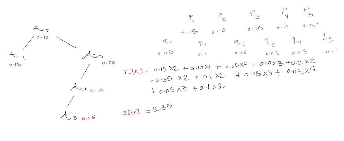
We store elements $A_{1} < A_{2} < \dots < A_{n}$. We are also given $p_{i}$, the probability of access for element $A_{i}$, and $q_{i}$, the probability of access for values between $A_{i}$ and $A_{i+1}$ (unsuccessful accesses). Also, we define $$\begin{gathered} A_{0} = -\infty, \quad A_{n+1} = \infty \ p_{0} = p_{n+1} = 0\end{gathered}$$
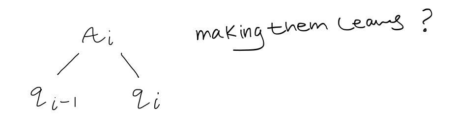
Let $T[i, j]$ be the root of the optimal tree on range $q_{i-1}$ to $q_{j}$. The cost of the tree rooted at $T[i,j]$ is $$\sum \text{probability of looking for one of these values (gaps) in the range} \times \text{the cost of doing this in that tree}$$
3. Dynamic programming
Observation
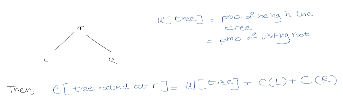
It will be handy to have $W[i,j]$, the probability of accessing any node/gap $q_{i-1}, \dots, q_{j}$ or $p_{i}, \dots, p_{j}$. $$W[i,j] = \sum_{k=i}^j p_{k} + \sum_{k= i-1}^j q_{k}$$ $$W[i, j+1] = W[i, j] + p_{j+1} + q_{j+1}$$ All the entries of $W[i,j]$ can be computed in $O(n^2)$ time. #final why are we adding the probabilities to get the cost? $$C[i,j] = \cases{0 \quad \text{if} \quad j = i-1 \ W[i, j] + \min_{r = i}^j (C[i, r-1] + C[r+1, j]) \quad \text{if} \quad i \leq j}$$ OPTIMAL-BST($p, q, n$) for $i \leftarrow 1$ to $n+1$ $C[i, i-1] \leftarrow 0$ $W[i, i-1] \leftarrow q_{i-1}$ for $l \leftarrow 1$ to $n$ for $i \leftarrow 1$ to $n - l +1$ $j \leftarrow i + l -1$ $C[i, j ] \leftarrow \infty$ $W[i,j] \leftarrow W[i, j-1] + p_{i} + q_{j}$ for $r \leftarrow i$ to $j$ $t \leftarrow C[i, r-1] + C[r+1, j] + W[i,j]$ if $t < C[i,j]$ $C[i,j] \leftarrow t$ $T[i,j] \leftarrow r$
Running time: $O(n^3)$ But $O(n^2)$ time is possible!
3. Splay trees
1. On accessing a node, we move (splay) it to the root by a sequence of local moves
2. Splaying
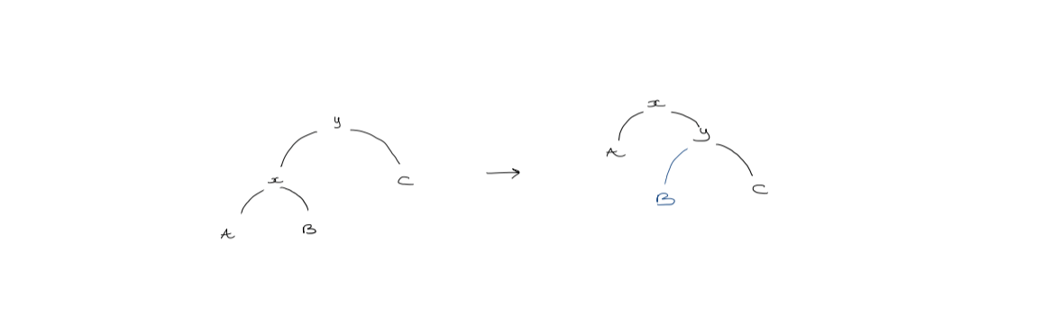
We let $x$ be a node being moved toward the root, $y$ be its parent, and $z$ be $y$'s parent. There are $3$ cases of splaying:
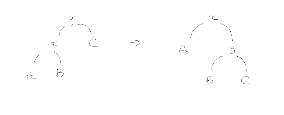
- Zig step
If $y$ is the root, we rotate $x$ so that it becomes the root (single rotation).
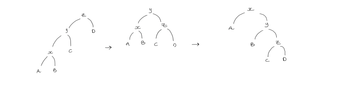
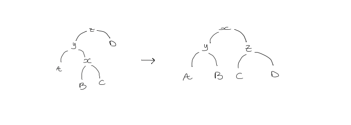
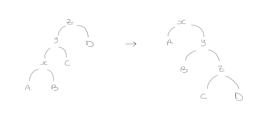
 2. Zig-zig step
If $y$ is not the root and $x$ and $y$ are both left or both right children, and we first rotate $y$ then rotate $x$.
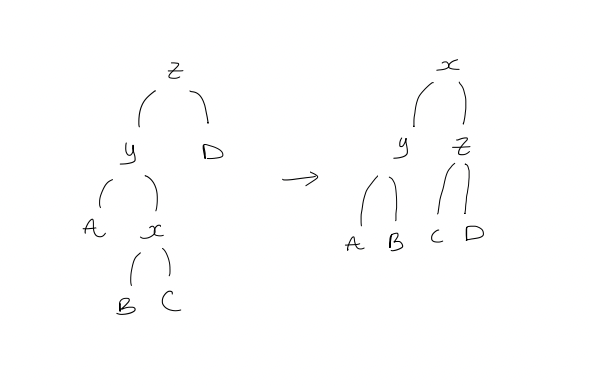
- Zig-zag step
If $y$ is not the root, and $x$ is a left child while $y$ is a right child, or vice versa, then we double rotate $x$.
 Running time analysis
- Splaying a node $x$ of depth $d$: $O(d)$
Example: single rotation of $x$ only (not splaying)
 Splaying
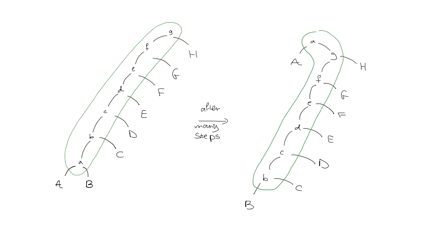
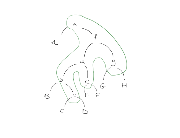 Intuition: splaying roughly halves the length of the access path
Definitions:
- $w(i)$ is the weight of item $i$ (positive)
- #final are items leaves? no
- $s(x)$ is the size of a node $x$ in the tree; sum of weights of all individual items in the subtree rooted at $x$
- $r(x)$ is the rank of node $x$; defined as $\log(s(x))$
- The potential, $\phi$, of the tree is the sum of the ranks of all its nodes
Note: $\phi_{i}$ is not necessarily nonnegative $$\sum_{i=1}^nC_{i} = \sum_{i=1}^m a_{i} + \phi_{0} - \phi_{m}$$ The cost if the number of rotations.
Access lemma: the amortized time to splay a tree with root $t$ at node $x$ is at most $$3(r(t) - r(x)) + 1 = O\left( \log\left( \frac{s(t)}{s(x)} \right) \right)$$ Proof:
If there are no rotations ($x$ happens to be $t$), then the bound is immediate (cost is $0$).
So, assume that there is at least one rotation and consider the first splaying step. There are three cases for this step
- Zig
- Zig-zig
- Zig-zag
Let $r_{0}(i)$, $r_{1}(i)$ and $s_{0}(i), s_{1}(i)$ represent the rank and size of node $i$ before and after the first step. Also, let $y$ be the parent $x$, $z$ be the parent of $y$.
- Zig
$y$ is the root, so $y = t$.
 The actual cost for a single rotation is just $1$. The amortized cost is
$$\begin{gathered} 1 + \phi_{1} - \phi_{0} = 1+ (r_{1}(x) + r{1}(y)) - (r_{0}(x) + r_{0}(y)) \\leq 1 + r_{1}(x) - r_{0}(x) \\leq 1 + 3(r_{1}(x) - r_{0}(x)) \end{gathered}$$
(we only include ranks of $x$ and $y$ because they're the only nodes that gain/lose descendants, the rank of $x$ increases while that of $y$ decreases)
- Zig-zig step
 Amortized cost is
$$\begin{gathered} 2 + r_{1}(x) + r_{1}(y) + r_{1}(z) - r_{0}(x) - r_{0}(y) - r_{0}(z) \ = 2+ + r_{1}(y) + r_{1}(z) - r_{0}(x) - r_{0}(y) & (\text{because } r_{1}(x) = r_{0}(z)) \ \leq 2 + r_{1}(x) + r_{1}(z) - r_{0}(x) - r_{0}(x) & (\text{because } r_{1}(x) \geq r_{1}(y), \ r_{0}(x) \leq r_{0}(y)) \ \end{gathered}$$
We now show
$$\begin{gathered} 2 + r_{1}(x) + r_{1}(z) - 2r_{0}(x) \leq 3(r_{1}(x) - r_{0}(x)) \iff r_{1}(z) + r_{0}(x) - 2r_{1}(x) \leq -2 \ r_{1}(z) + r_{0}(x) - 2r_{1}(x) \ = (r_{1}(z) - r_{1}(x)) + (r_{0}(x) - r_{1}(x)) \ \log\left( \frac{s_{1}(z)}{s_{1}(x)} \right) + \log\left( \frac{s_{0}(x)}{s_{1}(x)} \right) = \log\left( \frac{s_{1}(z)}{s_{1}(x)} \cdot \frac{s_{0}(x)}{s_{1}(x)}\right) \end{gathered}$$
Since $s_{1}(x) \geq s_{1}(z) + s_{0}(x)$,
$$\begin{gathered} \frac{s_{1}(z)}{s_{1}(x)} + \frac{s_{0}(x)}{s_{1}(x)} \leq 1 \end{gathered}$$
Then $$\frac{s_{1}(z)}{s_{1}(x)} \cdot \frac{s_{0}(x)}{s_{1}(x)} \leq \frac{1}{4}$$
Because, apparently, $\sqrt{ ab } \leq \frac{a+b}{2}$
Amortized cost is
$$\begin{gathered} 2 + r_{1}(x) + r_{1}(y) + r_{1}(z) - r_{0}(x) - r_{0}(y) - r_{0}(z) \ = 2+ + r_{1}(y) + r_{1}(z) - r_{0}(x) - r_{0}(y) & (\text{because } r_{1}(x) = r_{0}(z)) \ \leq 2 + r_{1}(x) + r_{1}(z) - r_{0}(x) - r_{0}(x) & (\text{because } r_{1}(x) \geq r_{1}(y), \ r_{0}(x) \leq r_{0}(y)) \ \end{gathered}$$
We now show
$$\begin{gathered} 2 + r_{1}(x) + r_{1}(z) - 2r_{0}(x) \leq 3(r_{1}(x) - r_{0}(x)) \iff r_{1}(z) + r_{0}(x) - 2r_{1}(x) \leq -2 \ r_{1}(z) + r_{0}(x) - 2r_{1}(x) \ = (r_{1}(z) - r_{1}(x)) + (r_{0}(x) - r_{1}(x)) \ \log\left( \frac{s_{1}(z)}{s_{1}(x)} \right) + \log\left( \frac{s_{0}(x)}{s_{1}(x)} \right) = \log\left( \frac{s_{1}(z)}{s_{1}(x)} \cdot \frac{s_{0}(x)}{s_{1}(x)}\right) \end{gathered}$$
Since $s_{1}(x) \geq s_{1}(z) + s_{0}(x)$,
$$\begin{gathered} \frac{s_{1}(z)}{s_{1}(x)} + \frac{s_{0}(x)}{s_{1}(x)} \leq 1 \end{gathered}$$
Then $$\frac{s_{1}(z)}{s_{1}(x)} \cdot \frac{s_{0}(x)}{s_{1}(x)} \leq \frac{1}{4}$$
Because, apparently, $\sqrt{ ab } \leq \frac{a+b}{2}$
Therefore, $$\begin{gathered} r_{1}(z) + r_{0}(x) - 2r_{1}(x) \ \leq \log\left( \frac{1}{4} \right) \ = -2 \end{gathered}$$' Hence, the amortized cost is $\leq 3(r_{1}(x) - r_{0}(x))$
- Zig-zag step
We double-rotate
 Amortized cost calculation:
$$\begin{gathered} & 2 + r_{1}(x) + r_{1}(y) + r_{1}(z) - r_{0}(x) - r_{0}(y) - r_{0}(z) \ & = 2 + r_{1}(y) + r_{1}(z) - r_{0}(x) - r_{0}(y) \ \text{Since } r_{0}(x) < r_{0}(y), \ & = 2 + r_{1}(y) + r_{1}(z) - 2r_{0}(x) \ \text{We now show } 2 + r_{1}(y) + r_{1}(z) - 2r_{0}(x) \leq 3(r_{1}(x) - r_{0}(x)) \ \text{This is equivalent to }\ & r_{1}(y) + r_{1}(z) + r_{0}(x) - 3r_{1}(x) \leq -2 \ \text{Note that } \ & r_{1}(y) + r_{1}(z) + r_{0}(x) - 3r_{1}(x) = \log\left( \frac{s_{1}(y)}{s_{1}(x)} \cdot \frac{s_{1}(z)}{s_{1}(x)} \right) + r_{0}(x) - r_{1}(x)\ \text{Since } s_{1}(x) \geq s_{1}(y) + s_{1}(z), \ & \leq \log \frac{1}{4} = -2 \end{gathered}$$ Suppose a splay operation requires $k > 1$ steps, then only the $k$th (last) step can be a zig step. The amortized cost of the whole splay operation is at most $$\begin{gathered} 3r_{k}(x) - 3r_{k-1}(x) + 1 + \sum_{j=1}^{k-1}(3r_{j}(x) - 3r_{j-1}(x)) \ = 3r_{{k}}(x) - 3r_{k-1}(x) + 1 + 3r_{k-1}(x) - 3r_{0}(x) \ = 3r_{k}(x) - 3r_{0}(x) + 1 \end{gathered}$$
The Balance Theorem states that given a sequence of $m$ accesses into an $n$-node splay tree $T$, the total access time is $O((m+n) \cdot \log(n) + m)$.
Proof:
We assign a weight of $\frac{1}{n}$ to each item. Then, $$\frac{1}{n} \leq s(x) \leq 1$$
Therefore, the amortized cost of any access is at most $$\leq 3 \left( \log(1) - \log\left( \frac{1}{n} \right) \right) + 1 = 3 \log(n)+1$$ The maximum potential of $T$ is $$\begin{gathered} \sum_{i=1}^n \log(s_{i}) \leq \sum_{i=1}^n \log(1) = 0 \end{gathered}$$ The minimum potential of $T$ is $$\sum_{i=1}^n \log(s_{i}) \geq \sum_{i=1}^n \log\left( \frac{1}{n} \right) = -n \log (n)$$ Therefore, $$\phi_{0} - \phi_{m} \leq 0 - (-n \log n) = n \log n$$ And the total actual cost is $$\begin{gathered} \leq m(3 \log n + 1) + \phi_{0} - \phi_{m} \ = 3m\log(n) + m + n \log n \ = O((m+n) \log n + m) \end{gathered} $$
But what does this mean?
$\rightarrow$ If we access $m \geq n$ times, the average cost per access is $\frac{O(m \log n + m)}{m} = O(\log n)$
The Static Optimality theorem states that given a sequence of $m$ access into an $n$-node splay tree, where each item is accessed at least once, then the total access time is $O\left( m+\sum_{i=1}^n q(i) \log\left( \frac{m}{q_{i}} \right) \right)$ where $q_{i}$ is the number of times item $i$ is accessed.
Proof:
We assign a weight of $\frac{q_{i}}{m}$ to each item $i$. Then, $$\frac{q(x)}{m} \leq s(x) \leq 1$$ The amortized cost of $n$ accesses is at most $$\leq 3 \left( \log(1) - \log\left( \frac{q(x)}{m} \right) \right) + 1 = 3 \log\left( \frac{m}{q(x)} \right)+1$$ And $$\phi_{0} - \phi_{m} \leq 0 - \sum_{i=1}^n\log\left( \frac{q(i)}{m} \right) = \sum_{i=1}^n \log\left( \frac{m}{q(i)} \right)$$ And the total actual cost is $$\leq 3 \sum_{i=1}^n q(i) \log\left( \frac{m}{q(i)} \right) + m + \sum_{i-1}^n \log\left( \frac{m}{q(i)} \right) \leq O\left( m + \sum_{i=1}^n q(i) \log\left( \frac{m}{q(i)} \right)\right)$$
We define the following as the entropy of access $\times m$ $$\sum_{i=1}^nq(i) \log\left( \frac{m}{q(i)} \right)$$
3. Update
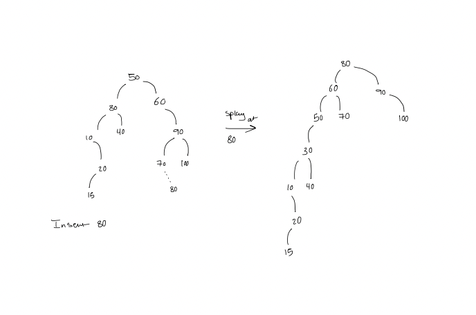
Insertion
- Insert as a new leaf
- Splay at the new node (the leaf that got turned into a node?)
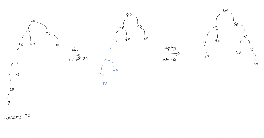
 Deletion
- Delete the node (creating 3 disconnected trees)
- Splay the largest value in its left subtree
- The right subtree becomes a subtree of the new root of the left subtree
- Replace the deleted node by the new root of these two subtrees connected together
- Splay at $x$'s parent
Self-Adjusting Lists
1. Problem: linear search
Given $n$ elements, and a key for an element, search for it by linearly iterating through the list.
Worst case: $n$ comparisons
Average case: If all elements have equal probability of search, then the expected time is $\frac{n+1}{2}$ in successful case and $n$ for an unsuccessful.
- How did we get $\frac{n+1}{2}$? $$\begin{aligned} \frac{1}{n}\cdot 1 + \frac{1}{n} \cdot 2 + \frac{1}{n} \cdot 3 + \dots + \frac{1}{n} \cdot n \= \frac{1}{n}(1+2+ \dots + n) \= \frac{n+1}{2} \end{aligned}$$
2. Real Questions
1. What if the probabilities of access differ?
Let $p_{i}$ be the probability of requesting element $i$.
2. What if these (independent) probabilities are not given?
3. How do solutions compare with the best we could do
3. Self-adjusting data structures - Adapt to changing probabilities
1. If probabilities are the same and independent, it doesn't matter how you change the structure
2. If both probabilities and list are fixed, minimize $\sum_{i=1}^n i p_{i}$
Greedy: element with the highest probability should be placed first.
Let $S_{opt}$ be the starting optimal solution.
3. How can we adapt to changes in probability or self-adjust?
Move elements forward as accessed.
Heuristics:
- Move-to-front (MTF): after an item is accessed, move it to the front of the list.
- Transpose (TR): After an item is accessed, exchange it with the immediate preceding item.
- Frequency count (FC): Maintain a frequency count for each item, initially $0$. Increase the count of an item by $1$ whenever it is accessed. Maintain a list such that the items are in decreasing order by frequency count.
4. Static optimality
1. Compare MTF to $S_{opt}$
2. Model
Start with an empty list. Scan for elements requested. If not present Insert (and change) as if found at the end of the list (then apply heuristic)
Cost: number of comparisons
3. The cost of MTF $\leq 2\cdot S_{opt}$ for any sequence of requests
Proof
Consider an arbitrary list, but focus on searches for $b$, $c$ (two arbitrary elements), and "unsuccessful comparisons" where we compare query value $b$ against $c$ or $c$ against $b$.
Assume the request sequence has $k$ $b$'s and $m$ $c$'s (no assumption on order of searches). Without loss of generality, assume that $k \leq m$.
$S_{opt}$ order is $c b$ and there are $k$ unsuccessful comparisons.
What order of requests maximizes this number under MTF?
Clearly, $C^{m-k}(bc)^k$.
There are $2k$ unsuccessful comparisons.
Under MTF, an unsuccessful comparison will happen whenever the request sequence changes, from $b$ to $c$ or $c$ to $b$.
Since each change involves a $b$ and each $b$ can be involved in at most two changes, the total number of such changes is $\leq 2k$.
This holds for any pair of elements, sum over all the total number of unsuccessful comparisons of MTF $$\leq 2 \cdot \dots \cdot S_{opt}$$
- 🔼 What is this?
We also observe that the total number of successful comparisons of MTF and the total number of successful comparisons of $S_{opt}$ are equal.
And the number of cost of MTF is at most $2 \cdot S_{opt}$.
4. This bound is tight.
Given $a_{1}, a_{2}, a_{3}, \dots , a_{n}$, we repeatedly ask for the last element in the list. So, the elements are requested equally often.
The cost of MTF is $n$ comparisons per search. But for the $S_{opt}$, every item has the same probability of being accessed, so the cost is $\frac{n+1}{2}$.
5. For some sequences, MTF does much better
Consider the following sequence of requests $$a_{1}^n \ a_{2}^n \dots a_{n}^n$$ The cost of $S_{opt}$ would be $\frac{n+1}{2}$
The cost of MTF would be $$\begin{aligned} \frac{(1+(n-1)) + (2+(n-1)) + (3+(n-1)) + \dots + (n + (n-1))}{n^2}\ = \frac{\frac{n(n+1)}{2} + n(n-1)}{n^2} \ = \frac{3}{2} - \Theta\left( \frac{1}{n} \right) \end{aligned}$$
5. Dynamic optimality
1. Online vs Offline
- Online: Must respond as requests come
- Offline: Get to see the entire schedule and determine how to move values
2. Competitive ratio of $Alg$
$=$ worst case of $\frac{\text{Online time of }Alg}{\text{Optimal offline time}}$
3. A method is "competitive" if this ratio is a constant
4. Model
- Search for or change element in position $i$: scan to location $i$ at cost $i$
- Free exchange: exchanges (swaps) between adjacent elements that are required to move element $i$ closer to the front are free of cost
- Paid exchange: any other exchange (swapping) between adjacent elements costs $1$
Before cost of self-adjusting
- $Access$: costs $i$ if element is in position $i$
- $Delete$: costs $i$ if element is in position $i$
- $Insert$: costs $n+1$ if $n$ elements are already there
5. Definitions
- Request sequence: $M$ queries, $n$ max data values
- Start with empty list
- Cost model for a search that ends with finding the element at position $i$ is $i +$ number of paid exchanges
- $C_{A}(S)$: the total cost of all operations for an algorithm $A$, not counting paid exchanges
- $X_{A}(S)$: number of paid exchanges $$X_{MTF}(S) = X_{TR}(S) = X_{FC}(S) = 0$$
- $F_{A}(S)$: number of free exchanges
Observation: $F_{A}(S) \leq C_{A}(S) - M$ After accessing the $i$th element, there are $\leq i - 1$ free exchanges.
Claim: $C_{MTF} \leq 2 C_{A}(S) + X_{A}(S) - F_{A}(S) - M$ for any algorithm $A$ starting with an empty set
Proof:
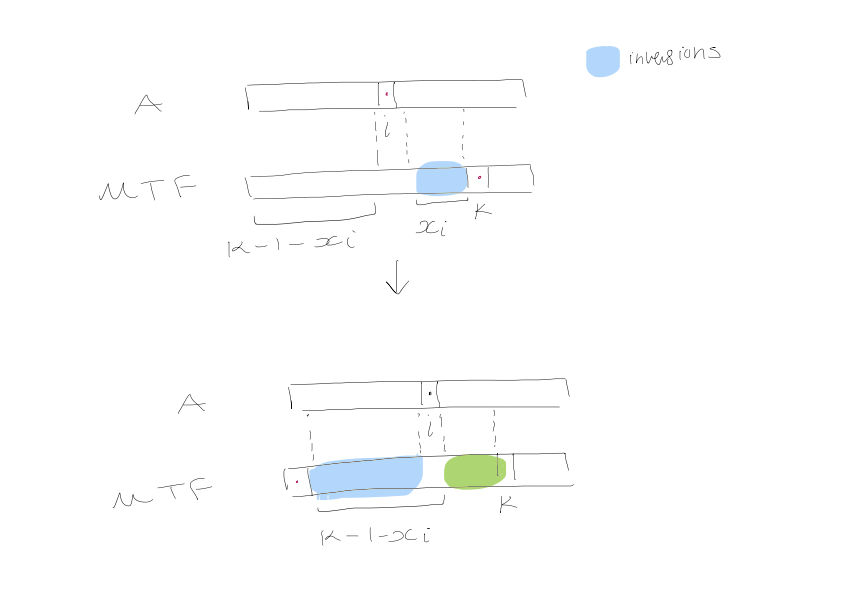
We run $A$ and $MTF$ in parallel, on the same request sequence $S$. The potential function $\phi$ is defined as the number of inversions* between $MTF$'s list and $A$'s list. Now, we bound the time of $access$.
Consider access by $A$ to position $i$ and assume we go to position $k$ is $MTF$'s list. Let $x_{i}$ be the number of items preceding the element in $MTF$'s list but not $A$'s list. So, the number of items preceding it in both lists is $k-1 - x_{i}$.
Moving the element to front in $MTF$'s list creates $k - 1 - x_{i}$ (between the element and those that used to precede it), and destroys $x_{i}$ inversions.
Amortized analysis: $$k + (k-1-x_{i}) - x_{i} = 2(k-x_{i}) - 1$$ Since $k-1-x_{i} \leq i-1$, we can conclude that $k-x_{i} \leq i$.
This gives us an amortized time of $\leq 2i - 1 = 2C_{A} - 1$ where $C_{A}$ is the cost of access for $A$ without exchanges (similar to insert/delete). An exchange by $A$ has $0$ cost to $MTF$, so the amortized time of an exchange by $A$ is increased in the number of inversions caused by exchange: $1$ for paid, $-1$ for free.
- #skipped for now ... So, the total amortized cost is $$2C_{A}(S) - M + X_{A}(S) - F_{A}(S)$$
Conclusion
MTF is $2$-competitive
$$\begin{aligned} T_{A}(S) &= C_{A}(S) + X_{A}(S) \ T_{MTF}(S) &= C_{MTF}(S) \ &\leq 2C_{A}(S) + X_{A}(S) - F_{A}(S) - M \ &\leq 2T_{A}(S) \end{aligned}$$ * An inversion is defined as any pair of elements that appear in different orders relative to each other in different lists.
Succinct Data Structures
1. Number of trees on $n$ nodes
- Binary trees
Catalan number $$C_{n} \equiv \frac{\binom{2n}{n}}{n+1}$$ 2. Ordinal trees
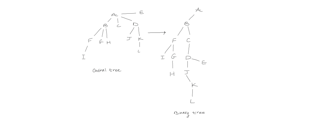
Defined as $$\text{child }1, \text{ child } 2, \text{ child } 3, \ \dots$$ To count the number of ordinal trees, we construct a mapping between ordinal trees and binary trees. The left child of every node will be the first child in the ordinal tree, but the the right child corresponds to the immediately right sibling.
2. Information-theoretic lower bound of representing a binary tree
- Definition of information-theoretic lower bound
Given a combinatorial object of $n$ elements where $u$ is the number of different such objects of size $n$, the information theoretic lower bound on the number of bits needed to represent such an object is $\log u$ bits (because we need to be able to distinguish the $u$ different objects).
- Binary trees $$\begin{aligned} \log C_{n} &= \log\left( \frac{(2n)!}{(n!)^2} \right) - \log(n+1) \ &= \log(2n)! - 2 \log n! - \log(n+1) \ &= 2n \log(2n) - 2n \log n + o(n) & \text{(Sterling's approximation)} \ & = 2n(\log(n+1)) - 2n \log n + o(n) \ &= 2n + O(n) \end{aligned}$$ Now, recall that $$\frac{\binom{2n}{n}}{(n+1)} \approx C \cdot \frac{2^{2n}}{n^{\frac{3}{2}}}$$ This allows us to turn $2n + O(n)$ into $$2n - \frac{3}{2} \log n + O(1)$$ $\rightarrow$ Trees can be represented in $2n$ bits!
But, can we still manage to navigate them when they're represented that succinctly?
3. Level-order representation of binary trees
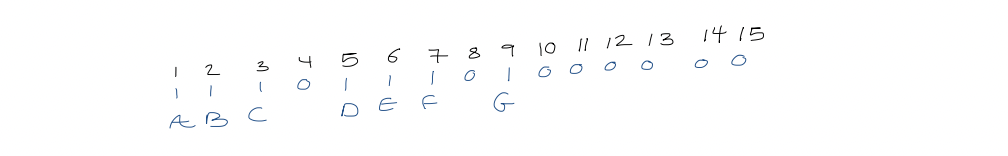
Append an external node for each missing child. For each node in level order, write $0$ if external, $1$ if internal
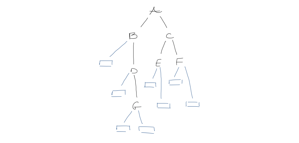
This takes $2n+1$ bits.
- Navigation
Claim: The left and right children of the $i$th internal node are at positions $2i$ and $2i+1$ in the bit vector.
Proof:
Induction on $i$.
This is clearly true for $i=1$ (root). For $i > 1$, by the induction hypothesis, the children of the $(i-1)$st internal node are at positions $2(i-1) = 2i - 2$ and $(2(i-1)) + 1 = 2i-1$.
Visually, this presents us with two cases:
- The $(i-1)$st and $i$th internal nodes are the same level
- The $(i-1)$st and $i$th internal nodes are not on the same level
Level ordering is preserved in children, i.e. $A$'s children precede $B$'s children in level order $\iff$ $A$ precedes $B$ in level order. All nodes between the $(i-1)$st internal node and the $i$th internal node are external nodes with no children, so the children of the $i$th internal node immediately follow children of the $(i-1)$st. So, they must be at positions $2i$ and $2i+1$.
Using the following definitions of rank and select $\text{rank}{1}(i) =$ the number of $1$s up to and including position $i$ $\text{select}{1}(j) =$ the position of the $j$th $1$-bit
We can identify each node by its position in the bit vector as $\text{left-child}(i) = 2 \cdot \text{rank}{1}(i)$ $\text{right-child}(i) = 2 \cdot \text{rank}{1}(i) + 1$ $\text{parent}(i) = 2 \cdot \text{select}_{1}\left( \left\lfloor \frac{i}{2} \right\rfloor \right)$
But how do we implement $\text{rank}$?
First, split the bit vector into $(\log^2n)$-bit superblocks
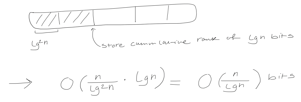 Then, split each superblock into $\frac{1}{2} \log n$-bit blocks
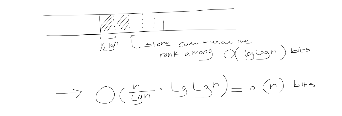 Use a lookup table for bit vectors of length $\frac{1}{2} \log n$. For any possible bit vector of length $\frac{1}{2} \log n$, and for each of its positions, store the answer.
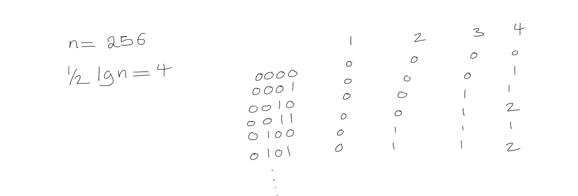
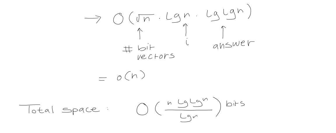 Finally, define $\text{rank}$ as $$\begin{aligned} \text{rank of superblock} \ + \quad \text{relative rank of block within superblock} \ + \quad \text{relative rank of element within block} \end{aligned}$$
Allowing us to computer it in $O(1)$ time. Note that we can follow a similar process for $\text{select}$.
Finally, define $\text{rank}$ as $$\begin{aligned} \text{rank of superblock} \ + \quad \text{relative rank of block within superblock} \ + \quad \text{relative rank of element within block} \end{aligned}$$
Allowing us to computer it in $O(1)$ time. Note that we can follow a similar process for $\text{select}$.
This allows us to conclude that we can represent a binary tree in $2n + o(n)$ bits, and access the $\text{left-child}, \ \text{right-child}, \ \text{parent}$ in $O(1)$ time.
Text Indexing Structures
1. Text Search
We are given an alphabet $\Sigma$ of size $\sigma$, a text string $T$ of length $n$ over $\Sigma$, and a pattern string $p$, we want to find the occurrences of $P$ in $T$.
2. String matching algorithms
- No preprocessing
- The obvious method: moving window
- $O(n + p)$-time solutions T
- Knuth-Morris-Pratt
- Boyer-Moore
- Rabin-Karp
3. Text indexing
- Preprocess a $T$-text index
- Each time a new pattern is given
4. Warm-up: trie
- Representing strings $T_{1}, T_{2}, \dots, T_{k}$
- A rooted tree with edges labelled with letters in $\Sigma$
- To represent strings as root-to-leaf paths in a trie, terminate them with a new letter $\$$ that is less than any symbol in $\Sigma$ > [!example] > Given ${ ana, ann, anna, anne }$, > >
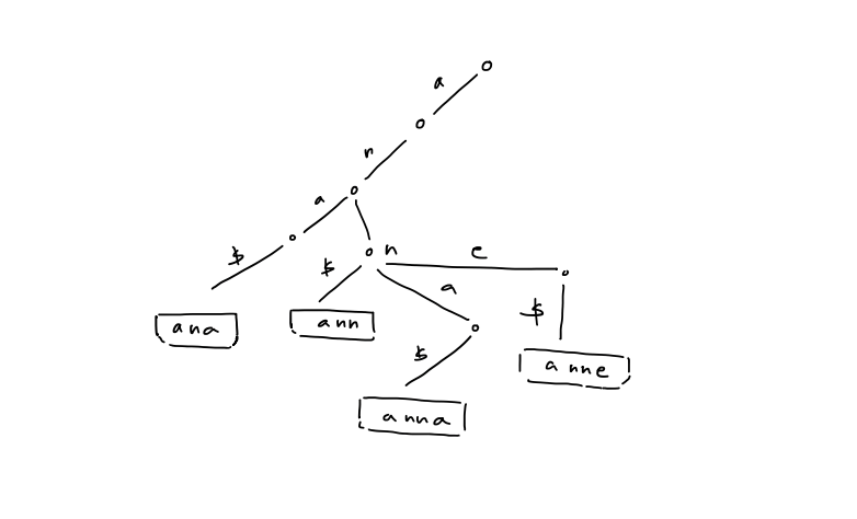 5. The in-order traversal of leaves is equivalent to a a sorting of the strings in lexicographical order 6. Check if $P$ is in ${ T_{1}, T_{2}, \dots , T_{k} }$ top-down traversal 7. If each node stores pointers to children in sorted order, then the number of nodes in the trie is $\leq \sum_{i=1}^k |T_{i}| + 1$ - Query time: $O(p \log \sigma)$ - Space: $O(n) +$ space form ${ T_{1}, T_{2}, \dots , T_{k} }$ 8. Compressed trie: contract non-branch paths to single edges > [!example] >
 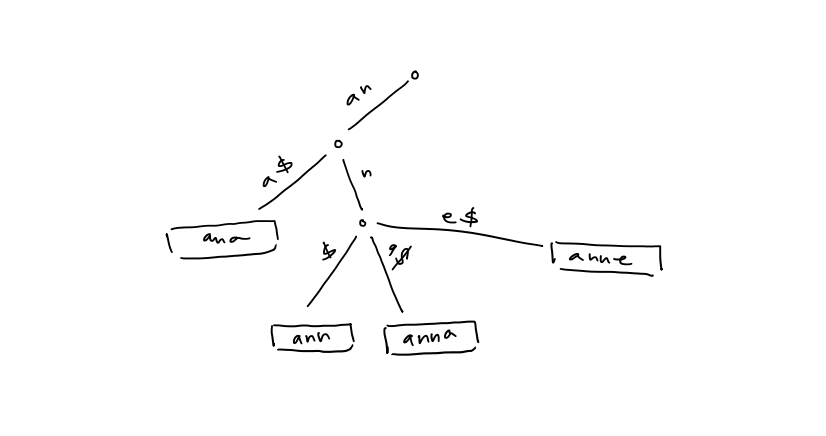 # 5. Suffix Tree 1. A compressed trie of all suffixes of $T \$$ > [!example] >
 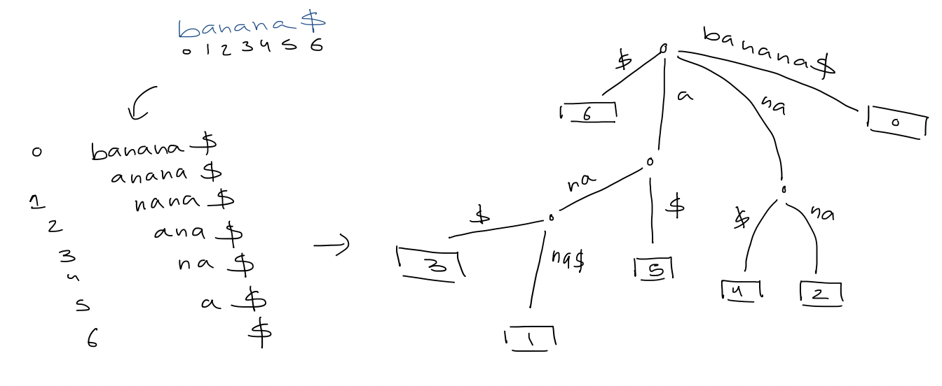 - $n+1$ leaves - Edge label = substring $T[i \dots j]$, store as two indices $(i, j)$ - Space: $O(n)$ 2. Text search - The search for $p$ gives a subtree whose leaves correspond to all occurrences of $p$ - If each node stores pointers to children in sorted order, the query time is $O(p \log \sigma)$ - If we use perfect hashing, the time becomes $O(p)$ - And, if we report all occurrences, the time is $O(p + occ)$ - [ ] #final what if the pattern does match any of the edges exactly (example: n instead of na) 3. Applications - Longest repeating substring in $T$ In $banana \$$, that would be $ana$.
We construct a suffix tree, then look for the branching node of maximum letter depth. When constructing a suffix tree, treat $\sigma$ as a constant, allowing us to bound the construction to $O(n)$ time.
- #final what does this mean? alphabet
Computing the letter depth in preorder traversal takes $O(n)$ time, too.
- #final because it uses DFS/BFS right?
6. Suffix array
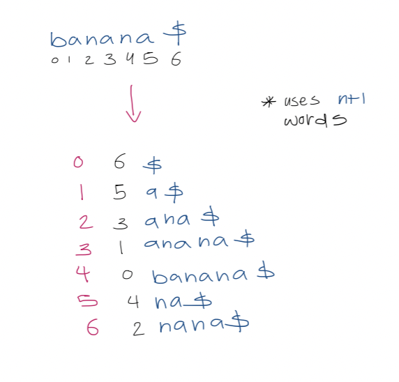
- Sort the suffixes of $T \$$, then just store the indices of the suffixes > [!example] > Note that the entries of the second column are the suffix array > >
 1. Text search with suffix array We use binary search over the array. This takes $O(\log(n+1)\cdot p)$ to determine where pattern $P$ of length $p$ occurs in $T$. 3. A simple accelerant Let $L, R$ be the left and right boundaries of the current search interval. We use a modified binary search which uses the midpoint to update $L$ or $R$. We also track $l$, the length of the longest prefix of $T[SA[L] \dots n]$ that matches $P$, and $r$, the length of the longest prefix of $T[SA[R] \dots n]$ that matches $P$. > [!example] > For $aba$, > > | $(L,R)$ | $(0,6)$ | $(0,3)$ | $(1,3)$ | $(1,2)$ | > | ------- | -------- | -------- | ------- | ------- | > | $(l,r)$ | $(0, 0)$ | $(0, 1)$ | $(1,1)$ | $(1,1)$ | Define $h$ as $\min(l, r)$. Observe that the first $h$ characters of $P, \ T[S[A] \dots n], \ T[SA[l+1] \dots n], \ \dots, \ T[SA[R] \dots n] \ = \ P[0 \dots h-1]$ So, when comparing in binary search, we can start from $P[h]$. 4. A super accelerant > [!example] > $lcp(2,3) = 3$ We call an examination of a character in $P$ redundant if that character has been examined before. Our goal is to reduce redundant character examination to be $\leq 1$ per iteration of the binary search such that the running time is $O(p + \log n)$ where the $p$ term is due to each non-redundant character examination. To achieve this goal, we need to do more preprocessing first. For each triple $(L, M, R)$ that can arise during binary search, we precompute $lcp(L,M)$ and $lcp(M,R)$. Since there are $(n+1) - 2$ unique midway points. Since there are two arrays indexed by $M$, this uses $2n-2$ total extra space. Let $Pos(i)$ represent the suffix starting at position $T[SA[i] \dots n]$. In the simplest case, in any iteration of the binary search, if $l = r$, then we compare $P$ to the suffix of the midway point $Pos(M)$, starting from $P[h]$, as before. In the general case, when $l \neq r$, we assume w.l.o.g, that $l > r$. We analyze the following three cases: 1. If $lcp(L,M) > l$, then the longest common prefix of suffixes $Pos(L)$ and $Pos(M)$ is larger than the longest common prefix between $P$ and $Pos(L)$.
 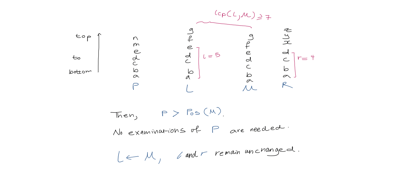 2. If $lcp(L, M) < l$,
 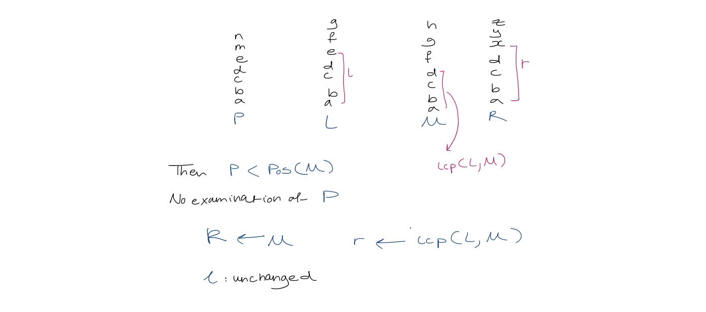 3. If $lcp(L, M) = l$, then $P$ agrees with $Pos(M)$ up to position $l-1$. Start comparisons from $P[l]$. - [ ] #final so, what happened to L and R here Compare middle, set middle to be left or right boundaries - [ ] #skipped I could probably figure this out if I tried longer ... Running time In the two cases where the algorithm examines a character during the iteration, the comparison starts with $P[\max(l, r)]$. Suppose $k$ characters of $P$ are examined in this iteration. Then there are $k-1$ matches, and $\max(l, r)$ increases by $k-1$. Hence, at the start of any following iteration, $P[\max(l, r)]$ may have already been examined but the next character in $P$ may not have been. Therefore, there are $\leq 1$ redundant character examinations per iteration.
 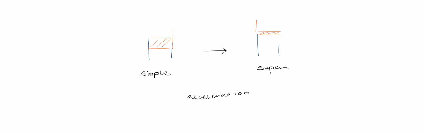 # 7. Construction 1. Suffix trees/arrays for Strings over a constant-sized alphabet can be constructed in $O(n)$ time. 2. Suffix trees/arrays for strings over an alphabet $\Sigma = { 1, 2, 3, \dots , n }$ can also be constructed in $O(n)$ time.
Mentions
- bzip2
Van Emde Boas Trees
1. Problem
1. Maintain an ordered set of elements to support
- Membership (search)
- Successor/predecessor
- Insert/delete
2. Most well-known solutions: balanced search trees
$\Theta(\log n)$ time for $O(n)$ space
3. Lower bound for membership (search) under the binary decision tree:
$\Omega(\log n)$
Binary decision tree model
- Any algorithm is modelled as a binary tree where each node is labelled $x < y$
- Program execution corresponds to a root-leaf-path
- Decision trees correspond to algorithms that only use comparisons to gain knowledge about input
Proof: Any binary decision tree for membership must have at least $n + 1$ leaves, one for each element + "not found". As a binary tree on $n+1$ leaves must have $\Omega(\log n)$, this lower bound applies.
4. "Counterexample": dynamic perfect hashing
Perfect hashing: every element can be searched for in $O(1)$ time but it doesn't support insert/delete.
Dynamic perfect hashing: can support insert/delete.
Membership: $O(1)$ worst-case Insert/delete: $O(1)$ amortized expected time Space: $O(n)$
5. Contradiction? Not really ... different machine models
RAM use input value as memory addresses, unlike binary decision tree model.
2. Model
1. Word RAM
- This model tries to model a realistic computer
- Word size $w \geq \log n$
- $O(1)$ "c-style" operations
2. Universe size: $u$
- Elements have values in the set ${ 0, 1, \dots, u-1 }$
- Elements fit in a machine word: $w \geq \log u$
3. Preliminary Approaches
1. Direct Addressing
Bit vector: $u = 16$, $n=4$, $S = { 1, 9, 10, 15 }$
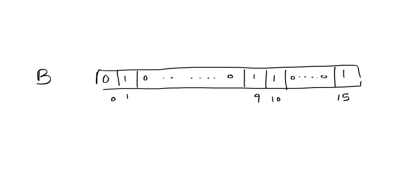 $Insert / Delete / Membership: O(1)$
$Successor / predecessor: O(u)$
$Insert / Delete / Membership: O(1)$
$Successor / predecessor: O(u)$
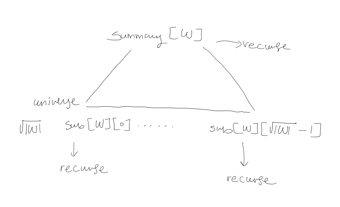
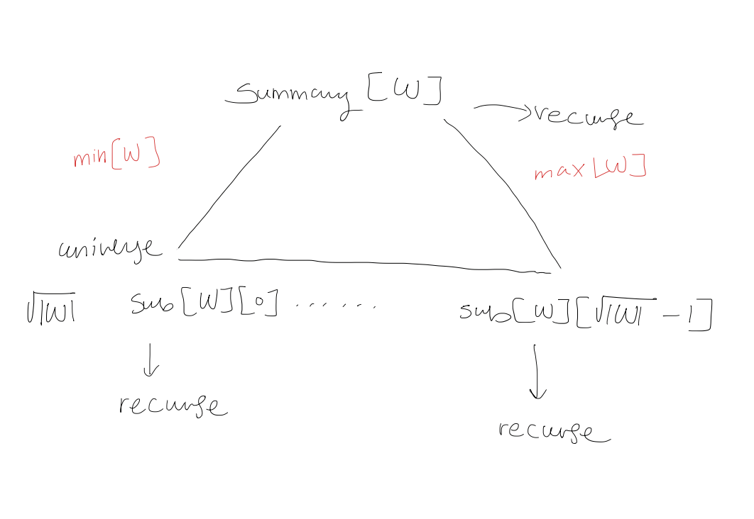
2. Carve into widgets of size $\sqrt{ u }$
$\rightarrow$ Assume that $u = 2^{2k}$
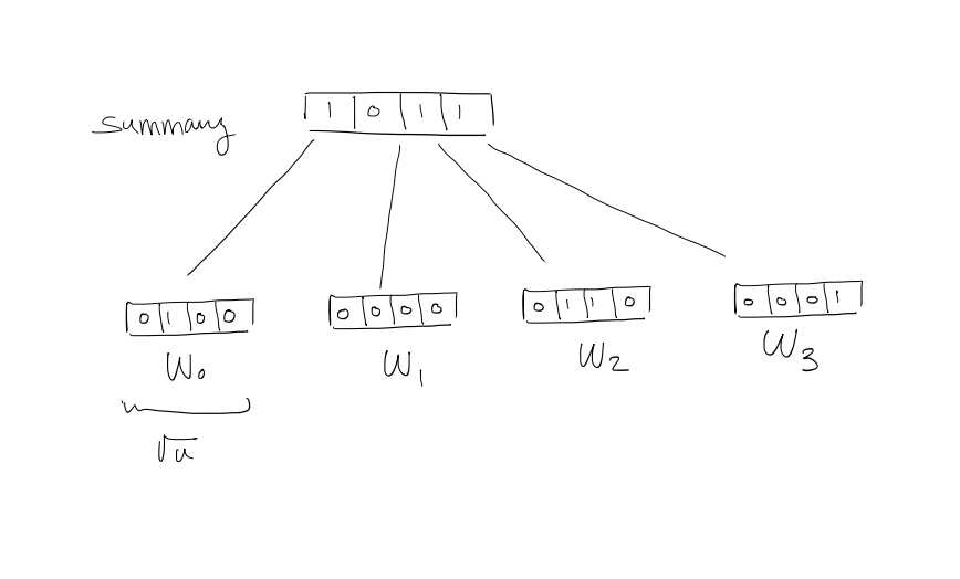 $W_{i}[j]$ denotes $i\sqrt{ u } + j$, $j=0, 1, \dots , \sqrt{ u } -1$
$Summary[j] = 1 \iff$ $W_{i}$ contains at least a $1$
$W_{i}[j]$ denotes $i\sqrt{ u } + j$, $j=0, 1, \dots , \sqrt{ u } -1$
$Summary[j] = 1 \iff$ $W_{i}$ contains at least a $1$
- $high(x) = \left\lfloor \frac{x}{\sqrt{ u }} \right\rfloor$
- $low(x) = x \mod{\sqrt{ u }}$
Both are $O(1)$.
- $x = high(x) \cdot \sqrt{ u } + low(x)$
- When $x$ is represented as a $\log u$-bit binary number, $high(x) =$ most significant $\frac{\log u}{2}$ bits $low(x) =$ lowest ...
Example $x = 9 \rightarrow 1001$ $high(x) = 10$ $low(x) = 01$ $Membership(x) = W_{high(x)}[low(x)] = W_{2}[1]$ Check if true!
$\text{successor}(x)$ Search to the right within $x$'s widget If we find a $1$, that position gives us the result Otherwise, search to the right within the summary If we find a $1$, that gives us the widget containing the Successor Scan that widget for the leftmost $1$
$\text{Insert/Delete}:$ widget, summary $\text{Insert:}O(1)$ because we simply set that but to $1$ and set its summary bit to $1$ if unset $\text{Delete}: O(\sqrt{ u })$: because we might have to scan the widget to see if there are any other $1$s, and unset the summary bit as needed
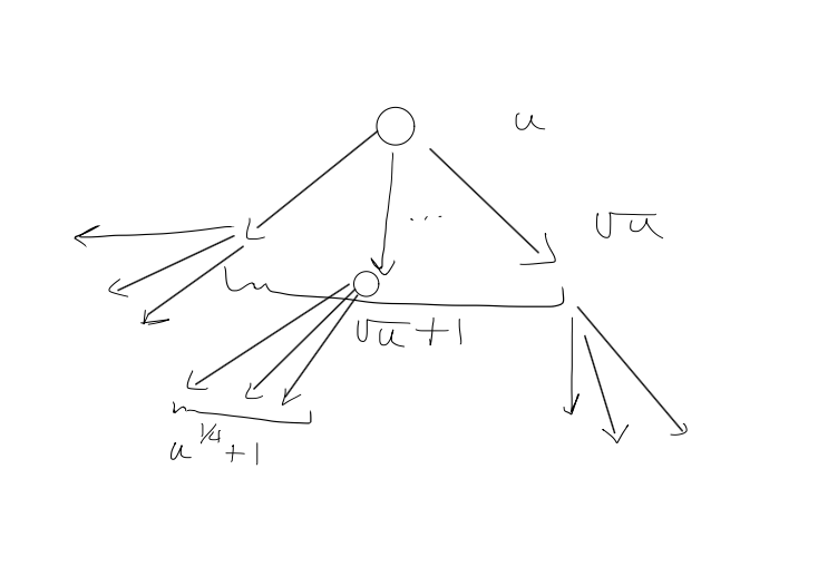
4. A recursive structure
1. $T(u) = T(\sqrt{ u }) + O(1)$
Let $m= \log u$, so that $u=2^m$
So that the recurrence becomes $$T(2^m) = T(2^{\frac{m}{2}}) + O(1)$$ Rename $S(m) = T(2^m)$ so that it becomes $$S(m) = S\left( \frac{m}{2} \right) + O(1)$$ Using the Master theorem, we can solve this as $$S(m) = O(\log m)$$ Change from $S(m)$ to $T(u)$ $$T(u) = T(2^m) = S(m) = O(\log m) = O(\log \log u)$$
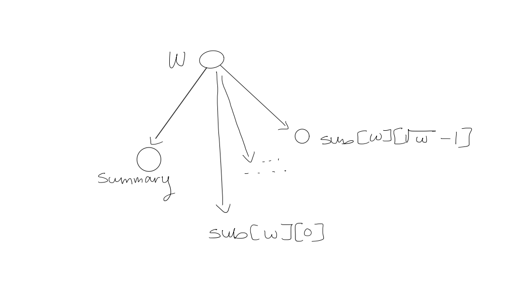
2. Widget $W$
 Base case: $W$ has $2$ bits
3. $\text{Member}(W,x)$
if $|W| = 2$ return $W[x]$ else return $\text{Member}(\text{sub}[W][\text{high}(x)], \text{low}(x))$
Since we are only making $1$ recursive call, the recurrence for this is $$T(u) = T(\sqrt{ u }) + O(1)$$ And so, the running time is $O(\log \log u)$
4. $\text{Insert}(W, x)$
if $|W| = 2$ $W[x] =1$ else $\text{Insert}(\text{sub}[W][\text{high}(x)], \text{low}(x))$ $\text{Insert}(\text{summary}[W], \text{high}(x))$
Since we make $2$ recursive calls, the recurrence for this is $$T(u) = 2T(\sqrt{ u }) + \Theta(1)$$ Let $m= \log u$, so that $u=2^m$ so that the recurrence becomes $$\begin{aligned} T(2^m) &= 2T(2^{m/2}) + \Theta(1) \ S(m) &= T(2^m) \ S(m) &= 2S\left( m/2 \right) + \Theta(1) \ S(m) &= \Theta(m) \ T(u) &= T(2^m) = S(m) = \Theta(m) = \Theta(\log u) \end{aligned}$$
5. $\text{Successor}(W, x)$
j $\leftarrow$ $\text{Successor}(\text{sub}[W][\text{high}(x)], \text{low}(x))$
if $j < \infty$ return $\text{high}(x)\sqrt{ |W| } + j$ else $i \leftarrow \text{Successor(Summary}[W], \text{high}(x))$ $j \leftarrow \text{Successor(sub}[W][i], -\infty)$
return $i \sqrt{ |W| } + j$
We make $3$ recursive calls. The running time is $\Theta((\log u)^{\log 3})$.
5. van Emde Boas Trees
1. Improvement 1: For each widget $W$, store $\min[W]$ and $\max[W]$
$\min[W] = \max[W] = -1$ if $W$ is empty
 $\text{Membership}: O(\log \log u)$
$\text{Successor}(W,x)$: if $x < \min[W]$ return $\min[W]$ else if $x \geq \max[W]$ return $\infty$ $W' \leftarrow \text{sub}[W][\text{high}(x)]$ if $\text{low}(x) < \max[W']$ return $\text{high}(x)\sqrt{ |W| } + \text{Successor}(W', \text{low}(x))$ else $i \leftarrow \text{Successor(Summary}[W], \text{high}(x))$ return $i \sqrt{ |W| } + \min[\text{sub}[W][i]]$
Which gives us $1$ recursive call in the worst case! $O(\log \log u)$
$\text{Insert(W, x)}$: if $\text{sub[W]}[\text{high}(x)]$ is empty $\text{Insert}(\text{Summary}[W], \text{high}(x))$ $\text{Insert(sub}[W][\text{high}(x)], \text{low}(x))$ if $x < \min[W]$ or $\min[W] = -1$: $\min[W] \leftarrow x$ if $x > \max[W]$ $\max[W] \leftarrow x$
2. Improvement: do not store $\min[W], \max[W]$ in any subwidgets of $W$
$\text{Membership}$: trivial change $\text{Successor}$: another trivial change
$\text{Insert(W,x)}$: if $\min[W] = \max[W] = -1$: $\min[W] \leftarrow \max[W] \leftarrow x$ else if $\min[W] = \max[W]$: $(\min[W], \max[W]) \leftarrow (\min(x, \min[W]), \quad \max(x, \max[W]))$ else: if $x < \min[W]$ $\text{swap}(x, \min[W])$ else if $x > \max[W]$ $\text{swap}(x, \max[W])$ $W' \leftarrow \text{sub}[W][\text{high}(x)]$ $\text{Insert}(W', \text{low}(x)) \quad (1)$ if $\max[W'] = \min[W']$: (2) $\text{Insert}(\text{summary}[W], \text{high}(x))$
Analysis If $(2)$ is true, then $(1)$ takes $O(1)$ time. $$\begin{gathered} T(u) = T(\sqrt{ u }) + O(1) \ O(\log \log u) \end{gathered}$$ $\text{Delete}(W, x)$: if $\min[W] = -1$: return if $\min[W] = \max[W]$: if $\min[W] = x$ $\min[W] \leftarrow \max[W] \leftarrow -1$ return if $\min[\text{summary}[W]] = -1$: if $\min[W] = x$: $\min[W] \leftarrow \max[W]$ else if $\max[W] = x$: $\max[W] \leftarrow \min[W]$ return if $\min[W] = x$: $j \leftarrow \min[\text{summary}[W]]$ $\min[W] \leftarrow \min[\text{sub}[W][j]] + j\sqrt{ |W| }$ $x \leftarrow \min[W]$ if $\max[W] = x$: $j \leftarrow \max[\text{summary}[W]]$ $\max[W] \leftarrow \max[\text{sub}[W][j]] + j\sqrt{ |W| }$ $x \leftarrow \max[W]$ $W' \leftarrow \text{sub}[W][\text{high}(x)]$ $\text{Delete}(W', \text{low}(x)) \quad \quad \quad \quad \quad \quad \quad \quad \quad \quad \quad \quad \quad \quad(1)$ if $\min[W'] = -1: \quad \quad \quad \quad \quad \quad \quad \quad \quad \quad \quad \quad \quad \quad (2)$ $\text{Delete}(\text{summary}[W], \text{high}(x))$
Time Analysis If $(2)$ is true, $(1)$ uses $O(1)$ time. $O(\log \log u)$.
Space Analysis $$S(u) = (\sqrt{ u } + 1)S(\sqrt{ u }) + \Theta(\sqrt{ u }) = O(u)$$ $\rightarrow\Theta(\sqrt{ u })$: pointers, min\max
What if $\sqrt{ u }$ is not an integer? $\rightarrow$ Then, each subwidget has size $\lceil \sqrt{ u} \rceil$ $$\begin{aligned} T(u) &= T(\lceil \sqrt{ u } \rceil ) + O(1) \ & \leq T(u^{2/3}) + O(1) \ &= O(\log \log u) \end{aligned}$$
6. X-fast Trie
1. Preliminary approach
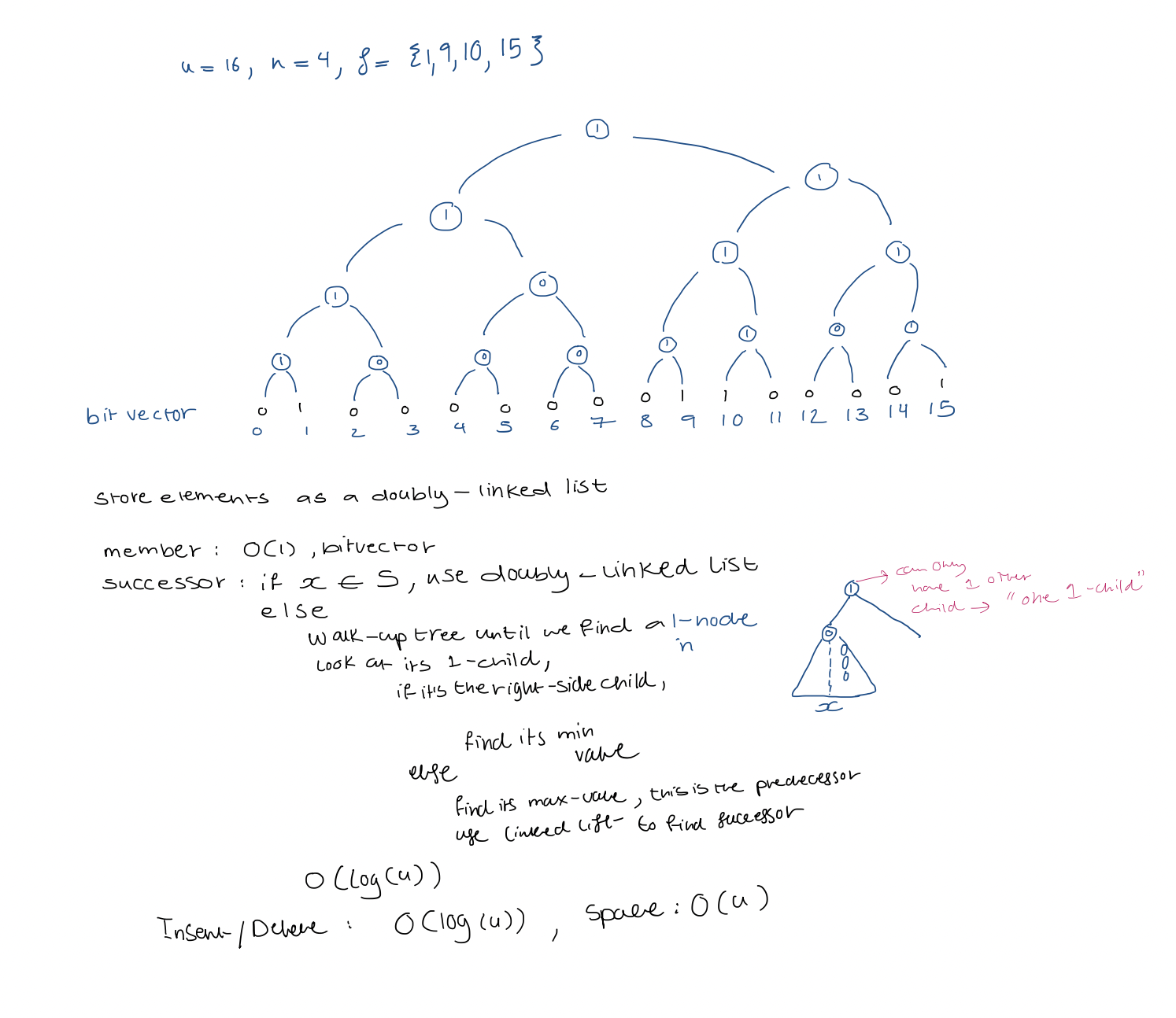
2. X-fast trie
- Do not keep the bitvector
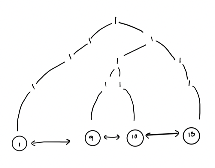
- Keep the doubly linked list
- Keep the $1$-nodes only
 Challenges:
 - $\text{successor}$: How to locate the lowest 1-node on the leaf-to-node path for a 0-leaf?
Solution:
a) Each ancestor of leaf $x$ corresponds to a prefix of $(x)_{2}$ (the binary representation of $x$)
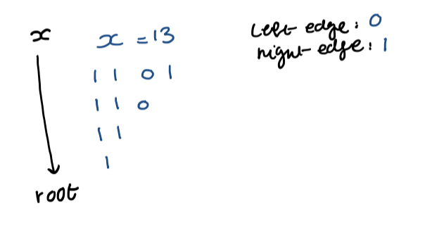 b) Using such a prefix as the key for any 1-node, we store it in a dynamic perfect hash table.
c) The lowest 1-node that is an ancestor of $x$ corresponds to the longest prefix of $x$ in the hash table
d) Binary search in prefixes of $x$ in $O(\log \log u)$ time
- If this node has a 1-child as its right child, store a descendant pointer to the smallest leaf of its right subtree ($\text{successor(x)}$)
- $\text{successor(x)}$: $O(\log \log u)$
- $\text{member: } O(1)$
- $\text{insert/delete : } O(\log u)$ amortized expected time
- space: list $O(n)$, hash table $O(n \log u)$, tree $O(n \log u)$
b) Using such a prefix as the key for any 1-node, we store it in a dynamic perfect hash table.
c) The lowest 1-node that is an ancestor of $x$ corresponds to the longest prefix of $x$ in the hash table
d) Binary search in prefixes of $x$ in $O(\log \log u)$ time
- If this node has a 1-child as its right child, store a descendant pointer to the smallest leaf of its right subtree ($\text{successor(x)}$)
- $\text{successor(x)}$: $O(\log \log u)$
- $\text{member: } O(1)$
- $\text{insert/delete : } O(\log u)$ amortized expected time
- space: list $O(n)$, hash table $O(n \log u)$, tree $O(n \log u)$
Dynamic perfect hashing on $m$ keys $O(m)$ space $O(1)$ worst-case $\text{member}$ $O(1)$ amortized expected $\text{insert/delete}$
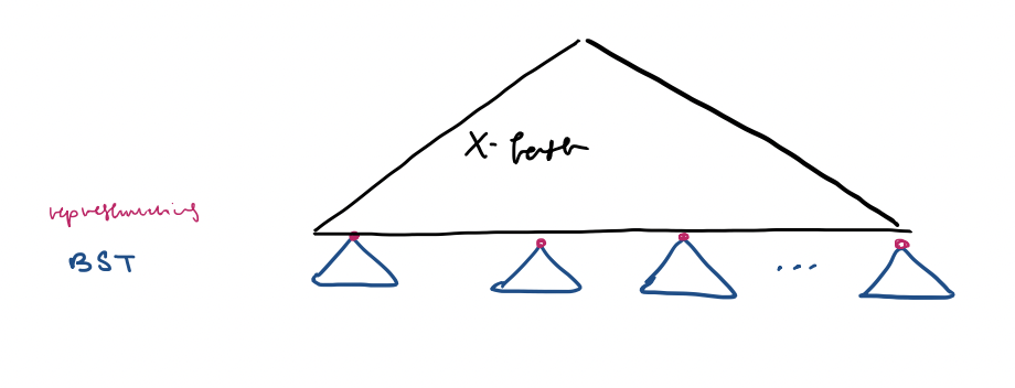
3. Y-fast trie
- Indirection
a) Cluster elements of $S$ into consecutive groups of size $\frac{1}{4} \log u \approx 2 \log u$
b) Store elements of each group in a balanced BST
c) Maintain a set of representative elements, one per group, stored in the X-fast trie structure
 A group's representative does not have to be in $S$ but it has to be strictly between the max element in the preceding groups and the min element in succeeding groups.
Space:
x-fast trie: $O((\text{number of elements}) \log u) = O\left( \frac{n}{\log u} \log u \right) = O(n)$
BSTs: $O(n)$
So, overall, $O(n)$
Time:
$\text{Member(x)}$
If $x$ is in the x-fast trie, it is not necessarily in $S$.
Search the corresponding binary balanced search tree for $x$. If we can find it, it must be in $S$. $O(\log \log u)$.
Else,
Find the predecessor and successor of $x$ in the x-fast trie. $O(\log \log u)$.
We check those two BSTs to look for $x$. $O(\log \log u)$.
$\text{Successor(x)}$: $O(\log \log u)$
$\text{Insert/Delete(x)}$
Use the x-fast trie to locate the group that $x$ is in.
Insert (or delete) $x$ into the balanced BST for that group.
When a group is of size $2 \log u$, split it. If it is $< \frac{1}{4} \log u$, merge it with an adjacent group (this might cause another split).
Split/merge: $O(\log u)$ amortized expected time
This takes $\Omega(\log u)$ inserts/deletes
Total: $O(\log \log u)$ amortized expected time
A group's representative does not have to be in $S$ but it has to be strictly between the max element in the preceding groups and the min element in succeeding groups.
Space:
x-fast trie: $O((\text{number of elements}) \log u) = O\left( \frac{n}{\log u} \log u \right) = O(n)$
BSTs: $O(n)$
So, overall, $O(n)$
Time:
$\text{Member(x)}$
If $x$ is in the x-fast trie, it is not necessarily in $S$.
Search the corresponding binary balanced search tree for $x$. If we can find it, it must be in $S$. $O(\log \log u)$.
Else,
Find the predecessor and successor of $x$ in the x-fast trie. $O(\log \log u)$.
We check those two BSTs to look for $x$. $O(\log \log u)$.
$\text{Successor(x)}$: $O(\log \log u)$
$\text{Insert/Delete(x)}$
Use the x-fast trie to locate the group that $x$ is in.
Insert (or delete) $x$ into the balanced BST for that group.
When a group is of size $2 \log u$, split it. If it is $< \frac{1}{4} \log u$, merge it with an adjacent group (this might cause another split).
Split/merge: $O(\log u)$ amortized expected time
This takes $\Omega(\log u)$ inserts/deletes
Total: $O(\log \log u)$ amortized expected time